Example 1d: Interpret relative moment tensor results

This example illustrates how to interpret relative moment tensors. It relies on the results of the previous example 1c.

First, we import everything we need for this tutorial to work.

import matplotlib.pyplot as plt
from matplotlib import cm
import numpy as np
from relmt import io, mt, utils
from pyrocko.moment_tensor import MomentTensor
from pyrocko.plot import beachball
from IPython.display import display # trick to show files in notebook

Group events by faulting type

First we load all events along the fault zone, for visualization, and the relative moment tensor catalog with the outliers removed.

# Relative moment tensors
mtd = io.read_mt_table("muji/result/mt_summary-auto-no_outliers-7640.txt")

# Reference moment tensors
mtd_ref = io.read_mt_table("muji/data/reference_mts.txt")

# Initial event table (pre subset selection)
evd = io.read_event_table("data/events.txt")

For interpretation, we group the moment tensors by faulting type, using the Kagan angle as a distance metric. The labels are sorted by the number of associated events while the unclustered events receive the label 0.

# Cluster labels in order of input catalog
labels, *_ = utils.mt_clusters(
    mtd,  # Moment tensors defined by their position in the list
    method="kagan",  # Cluster events by Kagan angle
    distance_matrix=None,  # Pre-computed distance matrix for large datasets
    max_distance=25,  # Maximal distance (Kagan angle) for one cluster
    min_ev=3,  # Minimum number of events to form a cluster
    link_method="weighted",  # Method to combine events
)

# List ob labels
llist = list(labels.values())

# Unique labels
ulab = sorted(set(llist))

print(f"Grouped events into {len(ulab)} faulting types:")
print(", \n".join([f"Type {lab}: {sum(llist==lab)} events" for lab in ulab]))

Grouped events into 5 faulting types:
Type 0: 9 events, 
Type 1: 48 events, 
Type 2: 23 events, 
Type 3: 22 events, 
Type 4: 19 events

Plot events in map view

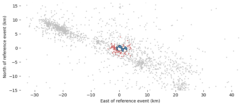
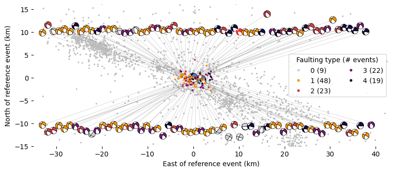
We will now plot the events on a map and color them by their faulting type. We will plot the catalog of the entire aftershock sequence in the background to get some tectonic context. The origin of our plot will be the location of the reference event. We first transform the data into practical coordinates and assign colors to the faulting types. We then set up the figure and plot everything.

evns = np.array(list(mtd.keys())) #  Event numbers

mtev = {evn: evd[evn] for evn in evns}  # Events with a moment tensor

# Select the reference event from the catalog
iref = 7640
rev = evd[iref]

# Origin north, east, depth coordinate
ned0 = np.array([rev.north, rev.east, rev.depth])

# Whole catalog and moment tensor north and east coordinates
ev_ned = (utils.xyzarray(evd) - ned0) * 1e-3
mt_ned = (utils.xyzarray(mtev) - ned0) * 1e-3

print("Spatial extent of events:")
print(
    f"North: {min(mt_ned[:, 0]) :.1f} to {max(mt_ned[:, 0]) :.1f} km, ",
    f"East: {min(mt_ned[:, 1]) :.1f} to {max(mt_ned[:, 1]) :.1f} km",
)

Spatial extent of events:
North: -3.0 to 3.9 km,  East: -4.0 to 4.2 km

Now we map faulting type to colors and make a legend

# Color map for faulting types
mtc = {
    lab: cm.inferno_r(frac) for lab, frac in zip(ulab, np.linspace(0.0, 0.9, len(ulab)))
}
mtc[0] = "lightgray"  # Gray for unclustered events

# Legend entries
handles = [
    plt.Line2D(
        [0],
        [0],
        marker="o",
        color="w",
        label=f"{lab} ({sum(llist==lab)})",
        markerfacecolor=col,
        markersize=5,
    )
    for lab, col in mtc.items()
]

We will first draw where we have started…

# Select the reference event from the catalog
iref = 7640
rev = evd[iref]

# Create the figure
fig, ax = plt.subplots(figsize=(8, 4), layout="constrained")

# Map coordinates
ax.set_xlim((-35, 43))
ax.set_ylim((-15, 16))
ax.set_aspect("equal")
ax.set_xlabel("East of reference event (km)")
ax.set_ylabel("North of reference event (km)")
ax.spines[:].set_visible(False)

# All events in the background
ax.scatter(*ev_ned[:, [1, 0]].T, s=2, color="silver", zorder=-5)

# Selected events
ax.scatter(*mt_ned[:, [1, 0]].T, s=2, color="indianred", zorder=0)

# Moment tensor plotting
mtsize = 2 # Size of the beachball in km

# Plot the reference moment tensors
for evn in [7508, 7640]:

    # Get the reference moment tensor and event
    momt = mtd_ref[evn]
    ev = evd[evn]

    # Event coordinates relative to reference event in km
    ned = (np.array([ev.north, ev.east, ev.depth]) - ned0) *1e-3

    # Convert to Pyrocko moment tensor
    thismt = MomentTensor(mt.mt_array(momt))

    # The beachball
    beachball.plot_beachball_mpl(
        thismt,
        ax,
        beachball_type="dc",
        size=mtsize,
        position=(ned[1], ned[0]),
        color_t="steelblue",
        linewidth=0.5,
        size_units="data",
    )

fig.savefig("relmt_begin.pdf")

… and now see how far we’ve got!

# Events with MTs colored by faulting type
ax.scatter(*mt_ned[:, [1, 0]].T, s=3, c=[mtc[lab] for lab in llist], zorder=5)

# The legend
ax.legend(title="Faulting type (# events)", handles=handles, ncol=2)

# Moment tensor plotting
mtsize = 1.5 # Size of the beachball in km
de = 0.8 * mtsize  # East offset for each MT

# East start coordinate of top and bottom MT row
east_top = -33
east_bot = -33

# North offset of top and bottom MT row
north_top = 10
north_bot = -10

# Sort from east to west for better display
esort = np.argsort(mt_ned[:, 1])

# top-bottom seperation north-coordinate
tbn = np.median(mt_ned[:, 0])

# Plot the moment tensors
for ii, ie in enumerate(esort):
    
    # Get name and faulting type of the event
    evname = evns[ie]
    lab = labels[evname]

    # Get moment tensor and event
    momt = mtd[evname]
    ev = evd[evname]

    # Event coordinates relative to reference event in km
    eve, evn = mt_ned[ie, [1, 0]]

    # Choose to plot in top or bottom row
    if evn > tbn:
        e = east_top
        n = evn + north_top
        east_top += de
    else:
        e = east_bot
        n = evn + north_bot
        east_bot += de

    # Highlight the reference event
    outline = "black"
    if evname == iref:
        outline = "red"

    # Convert to Pyrocko moment tensor
    thismt = MomentTensor(mt.mt_array(momt))

    # Color by faulting type
    color_t = mtc[lab]

    # Connecting line
    ax.plot([eve, e], [evn, n], color="gray", linewidth=0.2, zorder=-1)

    # The beachball
    beachball.plot_beachball_mpl(
        thismt,
        ax,
        beachball_type="dc",
        size=mtsize,
        position=(e, n),
        color_t=color_t,
        linewidth=0.5,
        edgecolor=outline,
        size_units="data",
    )
fig.savefig("relmt_finish.pdf")

display(fig)

Nice!

We see that 48 of the events (Type 1) are of the right-lateral WNW-striking transtensional type of the main shock and which align along the main fault trace delineated by all aftershocks (gray). 23 additional events of a similar type (Type 2), but with a weaker normal faulting component. Additionally we find 22 about (N)NW-striking transtensional events with a strong normal faulting component (Type 3). 19 W-striking odd to transpressional events (Type 4) are concentrated in the NE quadrant of the seismicity cloud and align along a W-E-striking structure. Additionally, we find 9 unclustered events (0).

Magnitude comparison

The relative moment tensors also provide a moment magnitude estimate(\(M_W\)) of each of the events. Let us compute it and compare to the local magnitude (\(M_L\)) provided in the catalog.

ml = [evd[evn].mag for evn in mtd]
mw = [mt.magnitude_of_vector(momt) for momt in mtd.values()]

fig, ax = plt.subplots()
ax.scatter(ml, mw, s=3, c="black", label="All events")
ax.scatter(evd[iref].mag, mt.magnitude_of_vector(mtd[iref]), s=5, c="red", label="Reference event")
ax.plot([1.5, 5], [1.5, 5], color="silver", linestyle="--", label="1:1", zorder=-1)
ax.set_xlabel("Catalog magnitude $M_L$ ($M_W$ for the two larges events)")
ax.set_ylabel("Moment magnitude $M_W$")
ax.set_aspect("equal")
_ = ax.legend()

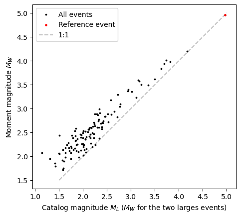
These are our newly determined relative moment magnitudes! The reference event plots on the 1:1 line, as it should be. The moment magnitude of the other reference event is also well reproduced. For the other events, it appears as if the local magnitude \(M_L\) consistently underestimated the seismic moment, especially at \(M_L < 3.5\).

Conclusion

This tutorial demonstrated the interpretation of relative seismic moment tensors. We learned how to judge the quality of a relative MT, and how to exclude outlying observations. We finally looked into the faulting types and moment magnitudes.