Example 1c: Relative amplitude measurement and computation of relative moment tensors

In this example we measure relative amplitudes on the aligned waveforms from the previous example. They provide the measurements we need to compute relative earthquake moment tensors. Amplitudes are measured in a specific frequency band, where we need to filter event combinations below the corner frequency of the largest event. relMT implements various algorithms to achieve this.

This notebook relies on the data previously created in the Example 1b.

Let us first change into the working directory…

%cd muji

/projects/restricted/relMT/relmt/src/relMT/examples/muji

… and import the modules required for this example.

from relmt import io, core
from itertools import cycle
import numpy as np
from matplotlib import pyplot as plt
from IPython.display import Image, display # trick to show files in notebook

Setting up a working configuration file

Let us set some configuration values that proved useful for this example.

The following configuration instructs relmt amplitude to do the following:

• Make sure the list of exculde files is the same as in the previous example (we will add one later that we do not want right now)

• Append the suffix “auto” to all files created

• Find automatic filter passbands for each event.

• Find the event low-pass frequency as the maximum in the velocity spectrum (the apparent corner frequency).

• Search for the maximum in the velocity spectrum inside the frequency band implied by a stress drop range between 0.1 and 10 MPa.

• Respecting the low-pass frequency, only include the frequency band with a signal-to-noise ratio > 0 dB.

• Measure relative amplitude ‘directly’, on the seismograms, between event combinations (pairs for P-waves, triplets for S-waves).

• Only allow event combinations with a common optimal bandpass with a dynamic range of at least 1dB.

In practice, we would open an editor and manipulate config.yaml accordingly.

config = io.read_config("config.yaml")

# List of files to read exluded events and phases, e.g. ['exclude.yaml']
# (list)
config["exclude_files"] = ['exclude.yaml', 'exclude-ecn.yaml']

# Suffix appended to files, naming the parameters parsed to 'amplitude'
# (str)
config["amplitude_suffix"] = "auto"

# Filter method to apply for amplitude measure. One of:
#    - 'manual': Use 'highpass' and 'lowpass' of the waveform header files.
#    - 'auto': compute filter corners using the "auto" options below
# (str)
config["amplitude_filter"] = "auto"

# The highpass filter corner allows not fewer than this  many signal periods
# within a phase window. Heuristic approach to eliminate low-frequency noise. A
# larger number means a higher highpass, narrower bandpass:
# highpass = `auto_highpass_periods` / (`phase_end` - `phase_start`).
# (float)
config["auto_highpass_periods"] = 2.0

# Method to estimate low-pass filter that eliminates the source time function. One
# of:
#    - 'corner': Estimate from apparent corner frequency in event spectrum.
#      Requires 'auto_lowpass_stressdrop_range'
#    - 'duration': Filter by 1/source duration of event magnitude. 
# (str)
config["auto_lowpass_method"] = "corner"

# When estimating the low-pass frequency of an event as the corner frequency
# (auto_lowpass_method: 'corner'), assume a stress drop within this range (Pa).
# When second value is less or equal first value, use a fixed stress drop of first
# value.
# ([float, float])
config["auto_lowpass_stressdrop_range"] = [1e5, 1e7]

# When estimating the low-pass frequency of an event as the corner frequency
# (auto_lowpass_method: 'corner'), use this near source S-wave velocity (m/s) to
# constrain the corner frequency estimate from spectrum
# (float)
config["auto_lowpass_vs"] = 3200

# Include frequencies with this signal-to-noise ratio to optimal bandpass filter.
# Respects low-pass constraint. If not supplied, do not attempt to optimize
# passband.
# (float)
config["auto_bandpass_snr_target"] = None

# Find the lowpass filter that is common to one phase of one event accross all 
# stations. Use the given quantile of the previously assigned lowpasses. `0`
# indicates minimum value, `0.5` median, `1` maximum value. The criterion is
# applied after the the individual waveform bandpasses are calculated or loaded
# from file.
# (float)
config["lowpass_event_phase_quantile"] = 0.2

# Method to measure relative amplitudes. One of:
#    - 'indirect': Estimate relative amplitude as the ratio of principal seismogram
#      contributions to each seismogram.
#    - 'direct': Compare each event combination separately.
# (str)
config["amplitude_measure"] = "direct"

# Minimum ratio (dB) of low- / high-pass filter bandwidth in an amplitude ratio
# measurement. When positive, discard observation outside dynamic range. When
# negative, lower the high-pass until the (positive) dynamic range is reached.
# (float)
config["min_dynamic_range"] = 1.0

config["ncpu"] = 20

config.to_file("config.yaml", overwrite=True)

INFO    : Configuration written to: config.yaml

Compute filter bands and relative amplitudes

We run relmt amplitude on the command line. To indicate that we would like to measure amplitudes on the waveforms stored in the align2/ directory, we parse the -a 2 flag. Computation of the filter bands and amplitudes takes a couple of (possibly 10) minutes.

! relmt amplitude -a 2

INFO    : Finding filter automatically
INFO    : No bandpass file found or overwrite option set. Computing.
INFO    : Saved bandpass to file: amplitude/bandpass-auto.yaml
INFO    : Collecting observations. This may take a while...
INFO    : Collected 22069 P- and 1742072 S-combinations
INFO    : Computing relative P-amplitudes...
INFO    : Computing relative S-amplitudes...

Plot the relative amplitudes

We can now have a look at the P amplitude observations with relmt plot-amplitude. The stations are sorted by azimuth relative to the event cluster centroid, and the event combinations are sorted by magnitude.

! relmt plot-amplitude amplitude/P-amplitudes-auto.txt --saveas tmp.png
display(Image("tmp.png"))

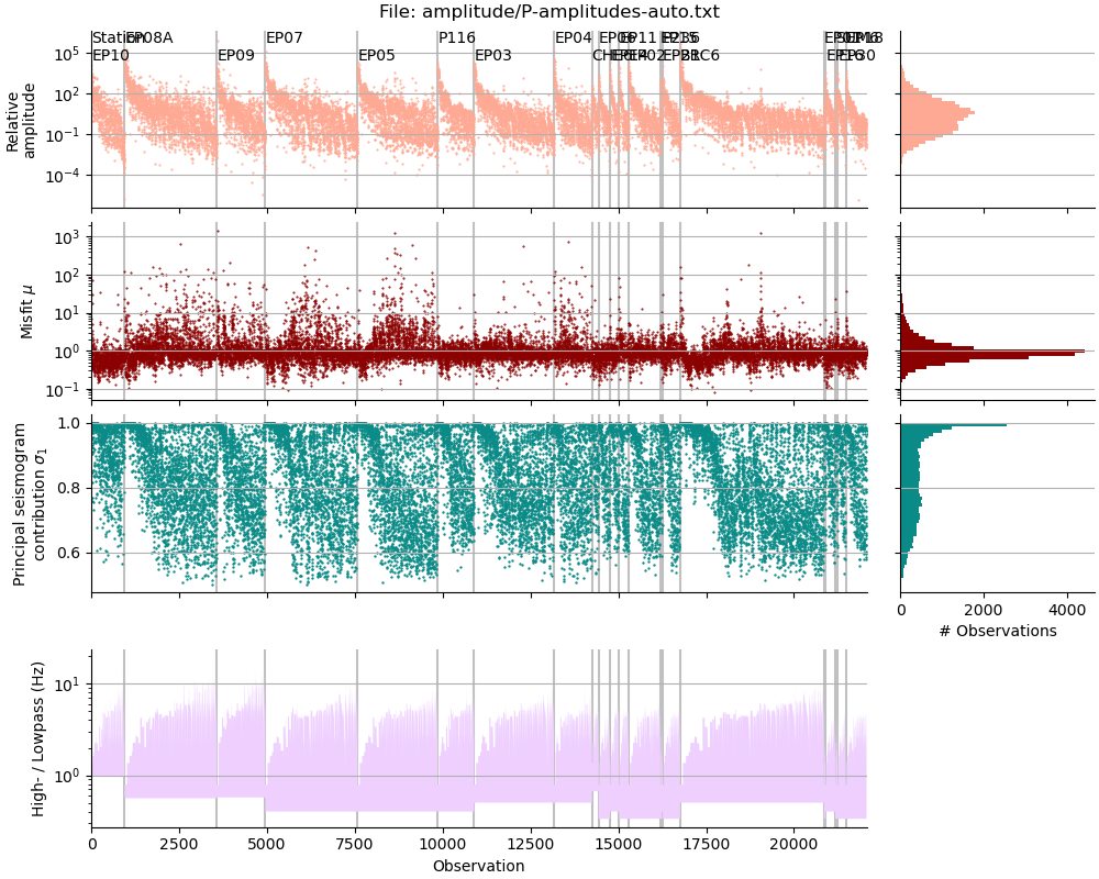
We see that there are just about 22,000 relative P-amplitude measurements. They range from about \(10^{-4}\) to to \(10^5\). The amplitude misfit scatters around 1, most values are slightly better (lower) than 1, and some stations (e.g.P116) yield arguably better misfits than others (e.g. EP09). High \(\sigma_1\) values indicate a high overall waveform similarity. The observations are sorted first by station distance, then by descending magnitude of the first event, and finally by ascending magnitude of the second event. This means we see compressions of the largest magnitude difference leftmost in each station panel. Note how the lowpass filter corner increases with smaller event magnitude and how the highpass filter is constant for one station

Next, we plot the S-wave amplitudes.

! relmt plot-amplitude amplitude/S-amplitudes-auto.txt --saveas tmp.png
display(Image("tmp.png"))

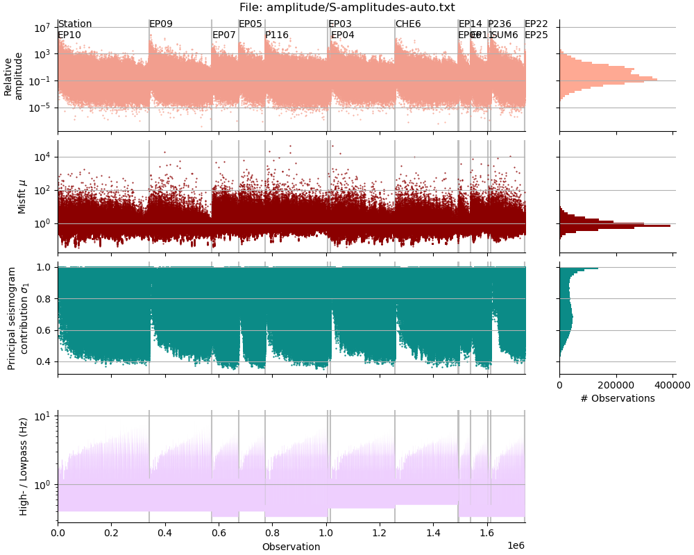
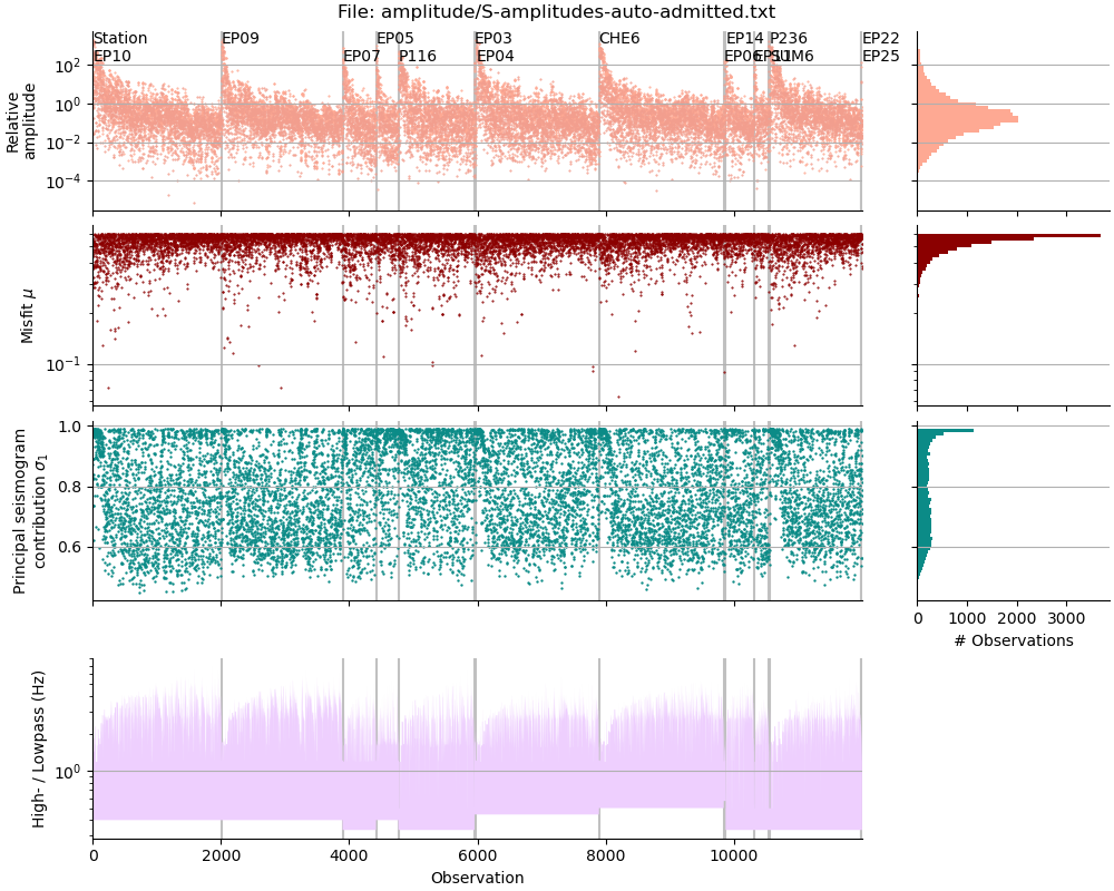
The S-amplitudes are much more abundant. The range of amplitudes as well as the scatter in misfit is comparable to the P-wave amplitudes.

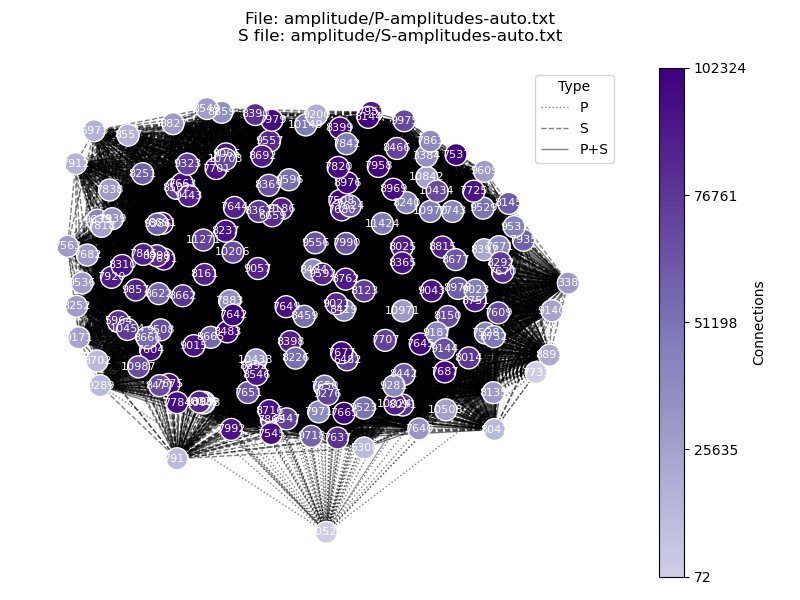
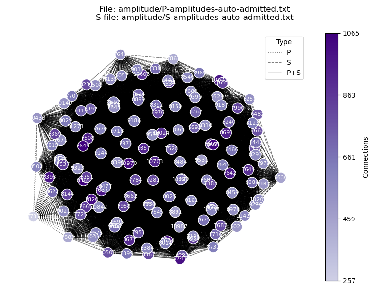
We can also have a look at how the amplitude measurements are connected with each other. The command below reads the P- and the S-amplitude files and illustrates which event is paired with which other event. We will see that some events have only a few dozen connections, while others have tens of thousands.

! relmt plot-connections amplitude/P-amplitudes-auto.txt -f amplitude/S-amplitudes-auto.txt -s tmp.png
display(Image("tmp.png"))

Admit amplitudes into the linear system of equations

We found relative amplitudes for 22,069 P-wave pairs and 1,742,072 S-wave triplets. We next admit the equations that should go into the linear system. The following configuration admits:

• relative P amplitudes with a misfit better than 0.95

• relative S amplitudes with a misfit better than 0.6

• relative S amplitudes with a \(\sigma_1\) value lower than 0.99

• events that are constrained by at least 10 equations

• events that have observations on at least 4 stations

• events that have a azimuthal gap lower than 270 degree

• both equations of each S observation triplet (representing the two polarization vectors),

• of the remaining P-equations, the 12,000 least redundant ones,

• of the remaining S-equations, the 24,000 least redundant ones, re-iterating 100 times.

After setting these values, we write the configuration to file and call relmt admit to write a new amplitude file, which now carries the suffix -admit. The next step also takes a few (possibly 2) minutes. For reproducibility we again make sure that we are only reading from the two exclude files we already know.

# List of files to read exluded events and phases, e.g. ['exclude.yaml']
# (list)
config["exclude_files"] = ['exclude.yaml', 'exclude-ecn.yaml']

# Suffix appended to the amplitude suffix, naming the quality control parameters
# parsed to 'relmt admit'
# (str)
config["admit_suffix"] = "admitted"

# Discard amplitude measurements with a higher misfit than this. Applies only to P
# amplitudes if 'max_s_amplitude_misfit' is given.
# (float)
config["max_amplitude_misfit"] = 0.95

# If given, discard S amplitude measurements with a higher misfit.
# 'max_amp_misfit' then only applies to P amplitudes.
# (float)
config["max_s_amplitude_misfit"] = 0.6

# Minimum shared path length fraction between events and station to allow an
# amplitude measurement. `1` indicates co-located events, `0` indicates
# inter-event distance equals event-station distance
# (float)
config["min_shared_path"] = 0.8

# Maximum first normalized singular value to allow for an S-wave reconstruction. A
# value of 1 indicates that S-waveform adheres to rank 1 rather than rank 2 model.
# The relative amplitudes Babc and Bacb are then not linearly independent.
# (float)
config["max_s_sigma1"] = 0.99

# Minimum number of equations required to constrain one moment tensor
# (int)
config["min_equations"] = 10

# Minimum number of stations required to constrain one moment tensor
# (int)
config["min_stations"] = 4

# Maximum azimuthal gap allowed for one moment tensor
# (float)
config["max_gap"] = 270

# Use two equations per S-amplitude observation (`False` only includes the one
# with the highest norm of the polarization vector).
# (bool)
config["two_s_equations"] = True

# Maximum number of P-wave equations in the linear system. If more are available,
# iteratively discard those with redundant observations, on stations with many
# observations, and with a higher misfit.
# (int)
config["max_p_equations"] = 12000

# As `max_p_equations`, but for S equations.
# (int)
config["max_s_equations"] = 24000

# When reducing the number of S-wave equations, rank observations iteratively this
# many times by redundancy and remove the most redundant ones. A lower number is
# faster, but may result in discarding less-redundant observations.
# (int)
config["equation_batches"] = 100

# Save it to file
config.to_file("config.yaml", overwrite=True)

! relmt admit

INFO    : Configuration written to: config.yaml
INFO    : Excluded 0 P-observations because stations or waveforms are excluded
INFO    : Excluded 0 more P-observations from exclude file
INFO    : Excluded 0 more P-observations due bad amplitude
INFO    : Excluded 9325 more P-observations due to high misfit
INFO    : Excluded 104 observations with shared path fraction smaller than 0.8.
INFO    : Excluded 0 S-observations because stations or waveforms are excluded
INFO    : Excluded 0 more S-observations from exclude file
INFO    : Excluded 0 more S-observations due bad amplitude
INFO    : Excluded 1258339 more S-observations due to high misfit
INFO    : Excluded 46355 more S-observations due high sigma1
INFO    : Excluded 27879 observations with shared path fraction smaller than 0.8.
INFO    : Excluding 25 events with too few equations, stations, or too large gap.
INFO    : Have 746302 S-equations, need to reduce by 722302
INFO    : Have 12313 P-equations, need to reduce by 313
INFO    : Selected 12000 P equations
INFO    : Selected 24000 S equations

Check the results

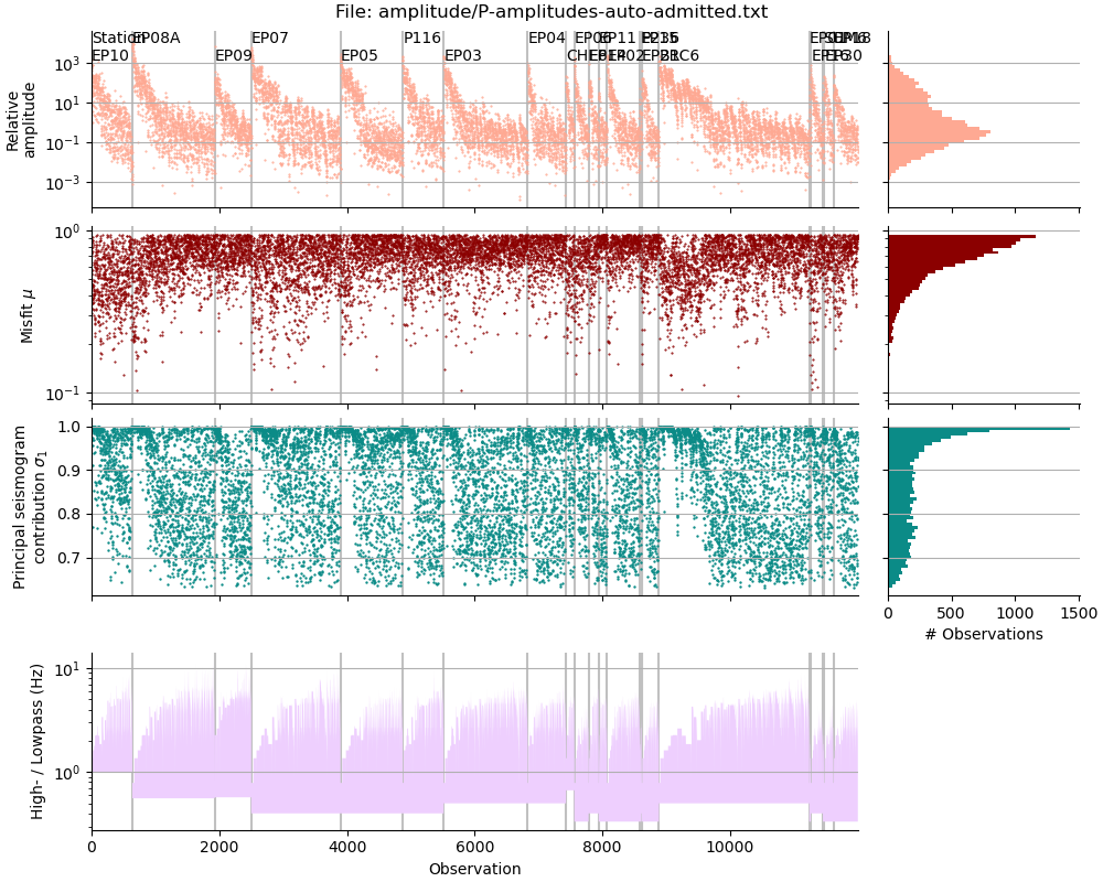
Each line in the newly created P amplitude file corresponds to one equation in the linear system, and each line in the S amplitude file to two (because two_s_equations is True). Each file has one header line.

! wc -l amplitude/[PS]-amplitudes*.txt

    12001 amplitude/P-amplitudes-auto-admitted.txt
    22070 amplitude/P-amplitudes-auto.txt
    12001 amplitude/S-amplitudes-auto-admitted.txt
  1742073 amplitude/S-amplitudes-auto.txt
  1788145 total

The created files are denoted with the amplitude suffix, they are called ‘amplitude/P-amplitudes-auto-admitted.txt’ and ‘amplitude/S-amplitudes-auto-admitted.txt’. As before, we can inspect them with relmt plot-amplitude and relmt plot-connections.

! relmt plot-amplitude amplitude/P-amplitudes-auto-admitted.txt --saveas tmp.png
display(Image("tmp.png"))

! relmt plot-amplitude amplitude/S-amplitudes-auto-admitted.txt --saveas tmp.png
display(Image("tmp.png"))

! relmt plot-connections amplitude/P-amplitudes-auto-admitted.txt -f amplitude/S-amplitudes-auto-admitted.txt -s tmp.png
display(Image("tmp.png"))

Solve the linear system

We will now read the file with the admitted amplitudes and build a linear system of equations according to the following configuration:

• Append the suffix “7508” to the result files, to indicate the number of the used reference event.

• Use event 7508 (the M 4.2) as the reference event.

• Weight the reference event with a weight of 1000

• Apply no constraint to the solution (solve for 6 MT elements)

• Apply the maximum weight of 1 to amplitude measurements with a misfit of 0.05

• Weight the worst accepted misfit 0.2

• Draw 100 bootstrap samples to detect unstable solutions

# Solve parameters
# ----------------
# 
# Suffix appended to amplitude and admit suffices indicating the parameter set parsed
# to 'solve'
# (str)
config["result_suffix"] = "7508"

# Event indices of the reference moment tensor(s) to use
# (list)
config["reference_mts"] = [7508]

# Weight of the reference moment tensor
# (float)
config["reference_weight"] = 1000

# Constrain the moment tensor. 'none' or 'deviatoric'
# (str)
config["mt_constraint"] = "none"

# Minimum misfit to assign a full weight of 1. Weights are scaled linearly from
# `min_amplitude mistfit` = 1 to `max_amplitude_misfit` = `min_amplitude_weight`
# (float)
config["min_amplitude_misfit"] = 0.05

# Lowest weight assigned to the maximum amplitude misfit
# (float)
config["min_amplitude_weight"] = 0.2

# Number of samples to draw for calculating uncertainties. If not given, do not
# bootstrap.
# (int)
config["bootstrap_samples"] = 100

config.to_file("config.yaml", overwrite=True)

INFO    : Configuration written to: config.yaml

The next command will build the system of linear equations, normalize the equations, apply weighting and solve it. Because we specified to draw 100 bootstrap samples in the configuration file, some additional bootstrap statistics will be computed as well.

! relmt solve

INFO    : Building linear system of 12000 P, 24000 S, and 6 reference equations.
INFO    : Computing norms and weights...
INFO    : Solving linear system of 840 variables and 36006 equations...
INFO    : Running lsmr...
INFO    : lsmr ended after 329 iterations with exit code 2
INFO    : Unweighted and weighted RMS are: 4.8e-11 and 7.2e-07 normalized Nm
INFO    : Computing 100 bootstrap samples...
INFO    : Saving full summary to: result/mt_summary-auto-admitted-7508.txt

Plot the results

The command relmt plot-mt facilitates plotting of a moment tensor file. It has options to sort and colour the beachball plots by a many different parameters, to highlight certain events and the double-couple component, and to save a plot to file. For full documentation, visit the help page.

The file that holds the MT solutions alongside the meta variables is result/mt_summary-auto-admitted-7508.txt. In the next plot we:

• Color the beachballs by the RMS of the weighted inversion residuals

• Sort the plots by input magnitude

• Highlight the reference event (7508) with a red outline

• Mark the nodal planes of double couple components > 20% with a line (for other events, the line is drawn between the positive and negative polarities on the focal sphere)

• Save the figure as a .png file.

! relmt plot-mt --color-by misfit --sort-by name --highlight 7508 --dc 0.2 --saveas ref7508.png result/mt_summary-auto-admitted-7508.txt
display(Image("ref7508.png"))

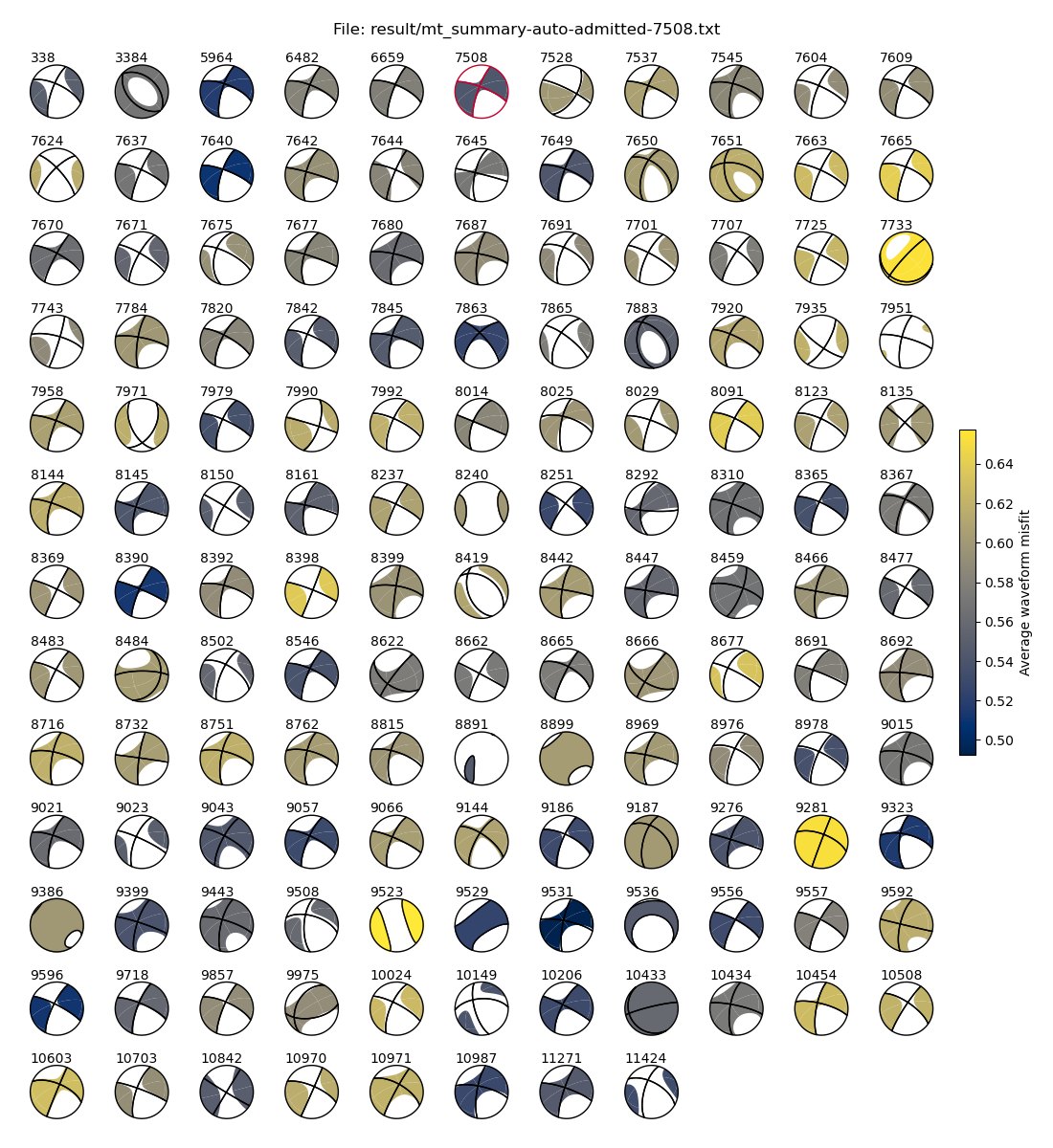
We have recovered 140 moment tensors. The double couple component of most of them resembles the reference MT and we see some normal faulting mechanisms and some MTs with a high CLVD or isotropic components. Some of the outlying MTs exhibit are qualitatively high average misfit, suggesting a poorer data basis for those

Before we start identifying outliers in the solution, let us first see what happenes if we select a different reference MT.

Try a different reference MT

We have another reference event available, event 7640 (M 5.0). Let us try and see how the results change when we use it as a reference. We change the configuration file by setting a new reference_mts list and append a changed result_suffix to the resulting files.

# Set event 7640 as the reference
config["result_suffix"] = "7640"
config["reference_mts"] = [7640]

# Save the configuration file
config.to_file("config.yaml", True)

! relmt solve

INFO    : Configuration written to: config.yaml
INFO    : Building linear system of 12000 P, 24000 S, and 6 reference equations.
INFO    : Computing norms and weights...
INFO    : Solving linear system of 840 variables and 36006 equations...
INFO    : Running lsmr...
INFO    : lsmr ended after 296 iterations with exit code 2
INFO    : Unweighted and weighted RMS are: 4.3e-13 and 6.4e-09 normalized Nm
INFO    : Computing 100 bootstrap samples...
INFO    : Saving full summary to: result/mt_summary-auto-admitted-7640.txt

The result file in question is now result/mt_summary-auto-admitted-7640.txt. We now color the MTs by the average correlation of the contributing waveform reconstructions. Both measures, average misfit and average correlation, are independent of the reference MT used so that the quality metrics can be transferred from one to the other.

! relmt plot-mt --color-by correlation --sort-by name --highlight 7640 --dc 0.2 --saveas ref7640.png result/mt_summary-auto-admitted-7640.txt
display(Image("ref7640.png"))

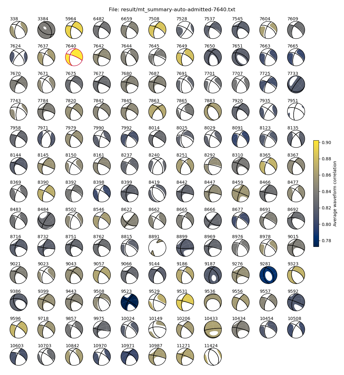
The results are qualitatively comparable, with most events showing strike-slip and subordinate normal-faulting mechanisms. There is a tendency for the entire data set to resemble reference moment tensor. We will next exclude outlying events and repeat the inversion.

Quantitative uncertainty analysis

We plot some misfit statistics of both event. First we define a function that creates a scatter plot of two variables with a corresponding histogram along each of the axes.

def plot_scatter(x, y, names, xlabel, ylabel, xlim=None, ylim=None, ishow=None):
    """Plot scatter with marginal histograms, show names of outliers."""

    # Plot 95% percentiles
    xq = np.quantile(x, 0.95)
    yq = np.quantile(y, 0.95)

    fig = plt.figure(figsize=(8, 8))

    gs = fig.add_gridspec(
        2, 2, width_ratios=(4, 1), height_ratios=(1, 4), wspace=0.05, hspace=0.05
    )

    # Scatter and historgram axes
    axs = fig.add_subplot(gs[1, 0])
    axx = fig.add_subplot(gs[0, 0], sharex=axs)
    axy = fig.add_subplot(gs[1, 1], sharey=axs)

    # Scatter plot
    axs.scatter(x, y, s=10)
    axs.axvline(xq, color="silver", zorder=-5)
    axs.axhline(yq, color="silver", zorder=-5)

    # Name outliers
    if ishow is None:
        # Show quantiles instead
        ishow = (x > xq) | (y > yq)

    for out in ishow.nonzero()[0]:
        axs.text(x[out], y[out], int(names[out]), ha="right")

    print("Worst 5%: " + ", ".join(f"{name :.0f}" for name in sorted(names[ishow])))

    # Histograms
    axx.hist(x, bins=30)
    axy.hist(y, bins=30, orientation="horizontal")

    # Clean up
    axx.tick_params(labelbottom=False)
    axy.tick_params(labelleft=False)
    axs.spines[["top", "right"]].set_visible(False)
    axx.spines[["top", "right", "left"]].set_visible(False)
    axy.spines[["top", "right", "bottom"]].set_visible(False)

    axs.set_xlabel(xlabel)
    axs.set_ylabel(ylabel)
    axs.set_xlim(xlim)
    axs.set_ylim(ylim)

We first look for outlying data with respect to the misfit and correlation measures. In out plots, high values will indicate worse data, so we instead of the correlation (cc) we will plot the anti-correlation (1 - cc)

mtfile = f"result/mt_summary-auto-admitted-7508.txt"

# Load the file
evns, mis, cc = np.loadtxt(mtfile, usecols=(0, 18, 19), unpack=True)

# Plot with the above defined function
xlab = "Average waveform misfit"
ylab = "Average waveform anti-correlation (1-cc)"
plot_scatter(mis, 1 - cc, evns, xlab, ylab)

Worst 5%: 7665, 7733, 8091, 8398, 8677, 9281, 9523, 10508, 10971

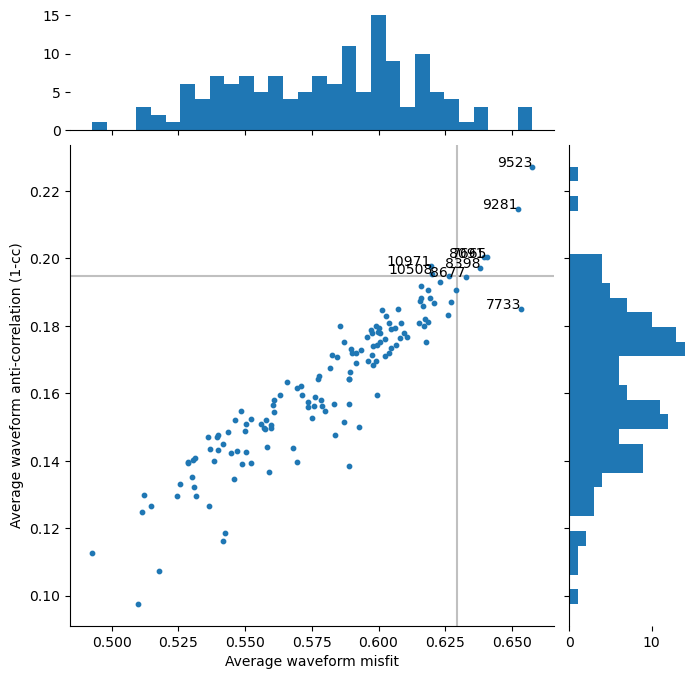
Based on this plot, we decide to exclude events with an anti-correlation larger than 0.25 (correlation lower than 0.75).

# Outlier definition
iout = (cc < 0.8) | (mis > 0.65)
excluded_events = sorted(evns[iout].astype(int).tolist())

print("Excluding events: " + ", ".join(str(evn) for evn in excluded_events))

# An empty exclude dictionary
exclude = core.Exclude()

# Append to exclude list and save
exclude["event"] = excluded_events
io.save_yaml("exclude-events.yaml", exclude)

Excluding events: 7665, 7733, 8091, 9281, 9523

Let us next investigate the stablity of the results. We do so by plotting the bootstapped Kagan angles (a measure of MT misorientation) against the bootstrapped moment RMS (a measure of MT consistency)

# Plot the two events one after another
plot_event = cycle([7640, 7508])

Exexute the next cell repeatedly to loop through the events

# Iterate through events
evn = next(plot_event)
mtfile = f"result/mt_summary-auto-admitted-{evn}.txt"

print(f"Plotting event {evn}")

# Load the file
evns, kagan_rms, moment_rms = np.loadtxt(mtfile, usecols=(0, 24, 25), unpack=True)

# Plot with the above defined function
xlab = "Bootstapped moment RMS (Nm/M0)"
ylab = "Bootstrapped Kagan angle RMS (°)"
plot_scatter(moment_rms, kagan_rms, evns, xlab, ylab, (0, 0.51), (0, 25))

Plotting event 7640
Worst 5%: 7883, 8484, 8692, 8891, 9386, 9523, 9529, 9531, 9536

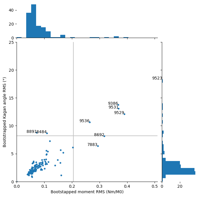
From comparing both misfit distributions, we see that reference event 7640 yields a overall better distribution of the Kagan angles, but refernce event 7508 a better moment RMS.

To decide which inversion is actually better, we will have a look at the actual inversion residuals. We here plot the weighted against the unweigted residuals

# Iterate through events
evn = next(plot_event)
mtfile = f"result/mt_summary-auto-admitted-{evn}.txt"

print(f"Plotting event {evn}")

# Load the file
evns, residual_rms, weighted_rms = np.loadtxt(mtfile, usecols=(0, 20, 21), unpack=True)

print(
    "Average unweighted and weighted RMS is: "
    f"{residual_rms.mean() :7.1e} and {weighted_rms.mean() :7.1e}"
)

# Plot with the above defined function
xlab = "Residual RMS (normalized Nm)"
ylab = "Weighted residual RMS (normalized Nm)"
plot_scatter(residual_rms, weighted_rms, evns, xlab, ylab, (0, 1.5e-6), (0, 1.5e-6))

Plotting event 7508
Average unweighted and weighted RMS is: 1.7e-07 and 2.3e-07
Worst 5%: 5964, 7508, 7604, 7640, 7677, 7733, 8237, 10971

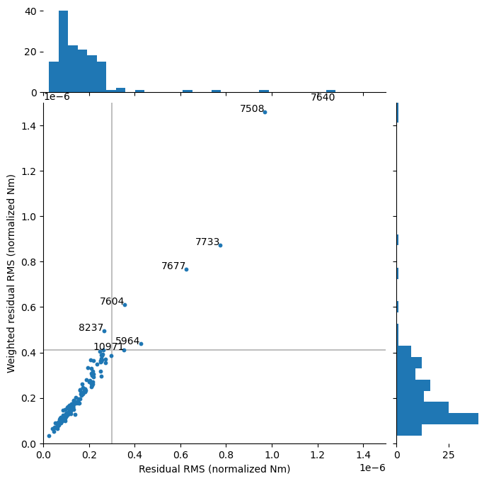
This argument suggests that reference event 7640 yields a better data fit than reference event 7508 and should therfore prefered.

We will therfore add the events that are poorly performing in terms of Kagan angle from reference event 7640 to the exclude list and solve the equation system again.

# Iterate through events
evn = 7640
mtfile = f"result/mt_summary-auto-admitted-{evn}.txt"

# Load the file
evns, kagan_rms = np.loadtxt(mtfile, usecols=(0, 24), unpack=True)

iout = kagan_rms > 5
excluded_events = sorted(evns[iout].astype(int).tolist())

print("Excluding events: " + ", ".join(str(evn) for evn in excluded_events))

# Append to exclude list and save
exclude["event"] += excluded_events
io.save_yaml("exclude-events.yaml", exclude)

Excluding events: 3384, 7671, 7865, 7883, 8135, 8484, 8692, 8891, 9386, 9523, 9529, 9531, 9536, 9592, 9975

We must remeber to add the new exclude file to the list of used exclude files. For outlier exclusion it is useful to only exclude events from a list after all other admission criteria have been applied. In this way, no new equations (possibly including additional outliers) are admitted into the equaion system. We do this by passing the --post flag to relmt admit.

# Read the config files
config = io.read_config("config.yaml")
# Add the exclude file
config["exclude_files"] += ["exclude-events.yaml"]

# Choose a new admission suffix
config["admit_suffix"] = "no_outliers"

# Select event 7640 as the reference
config["reference_mts"] = [7640]
config["result_suffix"] = "7640"

# Save the config file
config.to_file("config.yaml", overwrite=True)

# Admit the equations again
! relmt admit --post

# And solve the equation system
! relmt solve

INFO    : Configuration written to: config.yaml
INFO    : Excluded 0 P-observations because stations or waveforms are excluded
INFO    : Excluded 0 more P-observations due bad amplitude
INFO    : Excluded 9325 more P-observations due to high misfit
INFO    : Excluded 104 observations with shared path fraction smaller than 0.8.
INFO    : Excluded 0 S-observations because stations or waveforms are excluded
INFO    : Excluded 0 more S-observations due bad amplitude
INFO    : Excluded 1258339 more S-observations due to high misfit
INFO    : Excluded 46355 more S-observations due high sigma1
INFO    : Excluded 27879 observations with shared path fraction smaller than 0.8.
INFO    : Excluding 25 events with too few equations, stations, or too large gap.
INFO    : Have 746302 S-equations, need to reduce by 722302
INFO    : Have 12313 P-equations, need to reduce by 313
INFO    : Finally excluded -2359 P- and -3917 S-amplitudes from exclude file
INFO    : Selected 9641 P equations
INFO    : Selected 16166 S equations
INFO    : Building linear system of 9641 P, 16166 S, and 6 reference equations.
INFO    : Computing norms and weights...
INFO    : Solving linear system of 726 variables and 25813 equations...
INFO    : Running lsmr...
INFO    : lsmr ended after 185 iterations with exit code 2
INFO    : Unweighted and weighted RMS are: 6.9e-13 and 7.7e-09 normalized Nm
INFO    : Computing 100 bootstrap samples...
INFO    : Saving full summary to: result/mt_summary-auto-no_outliers-7640.txt

For comparisson, we once more compute the solution with reference event 7508, even though we already know that it yields a worse data fit.

# Select event 7508 as the reference
config["reference_mts"] = [7508]
config["result_suffix"] = "7508"

# Save to file
config.to_file("config.yaml", overwrite=True)

# Sovle the equation system
! relmt solve

INFO    : Configuration written to: config.yaml
INFO    : Building linear system of 9641 P, 16166 S, and 6 reference equations.
INFO    : Computing norms and weights...
INFO    : Solving linear system of 726 variables and 25813 equations...
INFO    : Running lsmr...
INFO    : lsmr ended after 213 iterations with exit code 2
INFO    : Unweighted and weighted RMS are: 7.8e-11 and 8.6e-07 normalized Nm
INFO    : Computing 100 bootstrap samples...
INFO    : Saving full summary to: result/mt_summary-auto-no_outliers-7508.txt

Let us first take a look at our preferred solution, this time sorted by magnitude.

! relmt plot-mt --sort-by magnitude --highlight 7640 --color-by boot-kagan --dc 0.2 --saveas 7640.png result/mt_summary-auto-no_outliers-7640.txt
display(Image("7640.png"))

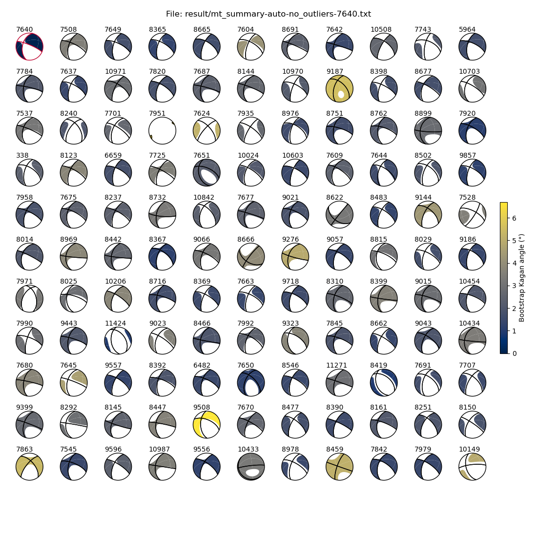
For comparison, we also look at the less preferd solution with the worse data fit.

! relmt plot-mt --sort-by magnitude --highlight 7508 --color-by boot-kagan --dc 0.2 --saveas 7508.png result/mt_summary-auto-no_outliers-7508.txt
image = cycle(("7508.png", "7640.png"))

By excecuting the next cell repretedly, we can examine the influence of the choice of reference MT.

# Excecute repeatedly to swap back and forth between both results
display(Image(next(image)))

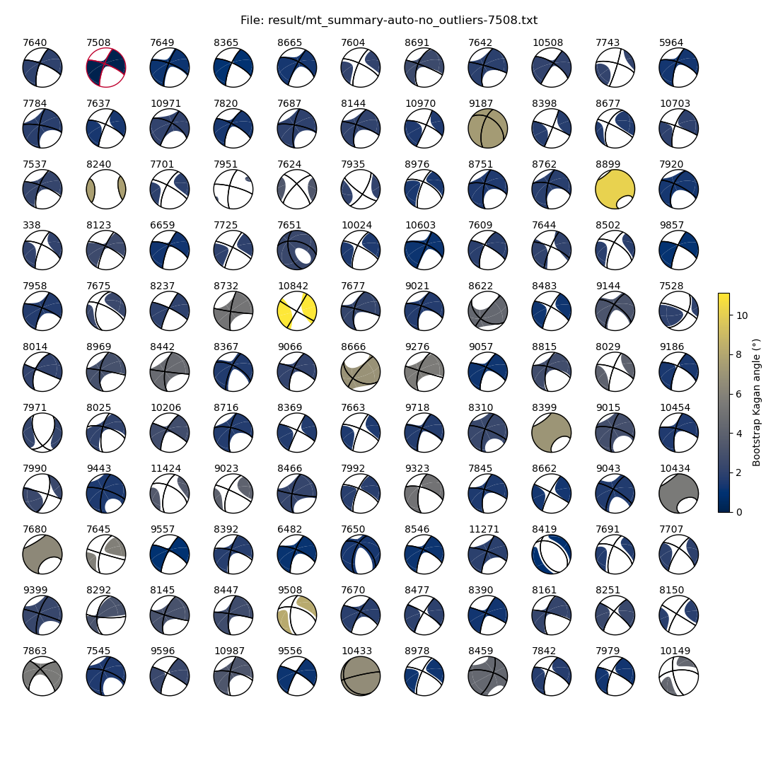
Reference MT 7640 yields overall slightly larger normal-faulting components, while 7508 yields larger strike-slip components. The faulting types and fault plane orientations, however, are preserved (e.g. normal faulting event 8419, 3rd row from the bottom and 3rd column from the left).

Importantly, reference event 7640 reproduces the absolute MT of event 7508 slightly better than vice versa, i.e. the normal faulting component of 7640 is not well reproduced when using 7508 as a reference, but the predominant strike-slip component of 7508 is still present when using 7640 as a reference.

The largest Kagan angle is larger using reference event 7508, because outlier exclusion was performed with reference event 7640.

Conclusion

In this notebook, we read aligned waveforms, determined optimal filter parameters, measured relative amplitudes, admitted certain amplitude mesurements into the linear system of equations and computed relative moment tenors for two different reference moment tensors. In the next notebook we will have a look at how to interpret the results.