Example 1a: Set up of an event subset of aftershocks#
In this example we will estimate relative moment tensors for a rather small subset of aftershock seismicity related to the 2016 M6.6 Muji earthquake in the Pamir highlands of Central Asia. The first notebook illustrates how to set up the input files for relMT.
This notebook relies on the results of the previous example. Please execute it before running this notebook.
from relmt import io, mt, utils, extra, core

from pathlib import Path
from warnings import filterwarnings
from IPython.display import Image, display # trick to show files in notebook

import matplotlib.pyplot as plt
from obspy import read_events, UTCDateTime, Inventory, Stream
from obspy.clients.fdsn import Client


# The networks considered here
nets = ["8H", "9H"]

def netcode(stacode):
    """Network code of a station"""

    # All 8H stations start with "EP"
    if stacode.startswith("EP"):
        return "8H"

    # All 9H stations that are not 8H have a "6" at the end
    if stacode[-1] == "6":
        return "9H"

    # We do not consider the other networks present
    return ""
Initialize the project#
We begin by initializing the folder structure though a call to relmt init. Let’s call the project like the mainshock: “muji”, and see what was created using ls. In the following lines, the exclamation mark ! indicates that the commands are run on the command line, using the shell as a interpreter. Indeed, relMT is intended to be used directly from the terminal.
! relmt init muji
! ls muji/*
INFO    : Configuration written to: muji/config.yaml
INFO    : Configuration written to: muji/data/default-hdr.yaml
INFO    : Working directory is complete: muji
muji/config.yaml  muji/exclude.yaml

muji/align1:

muji/align2:

muji/amplitude:

muji/data:
default-hdr.yaml

muji/result:
We see the configuration file config.yaml and the exclude file exclude.yaml. The directories data/, align1/, align2/, amplitude/ and result/ will be populated while we work on the project.
In this example we will start from scratch. This means we will create the necessary files from raw seismograms and arrival time picks, as it is often the case when starting a new project.
Extraction of the event and MT subsets#
Let us assume we would be interested in learning about the structure of the fault zone in between the two asperities that broke in the 2016 M6.6 Muji earthquake. Consider Fig. 6 of Bloch et al. (2023, GJI). We here want to work on the event subset marked by the bright red circle:
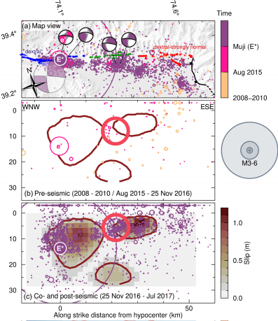
Two full moment tensors are available. There is more seismicity, occurring before as well as after the main shock. Let us extract the events that are located within 5 km from the largest aftershocks. From the figure we can see that the two events for which we have an MT available are located between 39.15˚N and 39.3˚N and 74.1˚E and 74.6˚E. Let’s see where we find those events in the MT file
! awk '$3 > 74.1 && $3 < 74.6 && $4 > 39.15 && $4 < 39.3 {print NR, $1, $2, $3, $4, $5, $6}' ext/2022-007_Bloch-et-al_moment_tensor_catalog_correct_norm_v2.0.txt
25 2016/11/25 19:46:20 74.29494 39.19792 6 4.2
26 2016/11/26 09:23:27 74.27384 39.20200 6 5.0
The events occurred on the 25. and 26. November 2016 and had magnitudes of 4.2 and 5.0. The first column indicates that we find the events in the 28th and 29th line of the provided MT file (1-based indexing). Remember that the input file has 4 header lines and Python uses 0-based indexing. That means, we are looking for the MTs at position 23 and 24 in the relMT file.
# Input files
evinf = "data/events.txt"
mtinf = "data/reference_mts.txt"

# Indices of reference events (0-based indexing)
irefs = [23, 24]

evd = io.read_event_table(evinf)
mtd = io.read_mt_table(mtinf)

refids = [list(mtd)[i] for i in irefs]

print("The reference events are: ", refids)
for refid in refids:
    print(f"Event {refid} ({evd[refid].name}): Mw {mt.magnitude_of_vector(mtd[refid]):.2f}")
The reference events are:  [7508, 7640]
Event 7508 (20161125194617): Mw 4.17
Event 7640 (20161126092323): Mw 4.95
The event times and magnitudes in the catalog agree with the one in the MT file. We have selected the correct events.
Let us find the events that are within 5km of Event 7640 and save them to the project directory.
# The event coordinates are the first three elements of the event tuple
xyz0 = evd[7640][:3]

dist = 5000  # m

iin = [
    evn for evn, ev in evd.items() if utils.cartesian_distance(*xyz0, *ev[:3]) < dist
]

evsub = {evn: evd[evn] for evn in iin}
mtsub = {evn: mtd[evn] for evn in mtd if evn in iin}

print(f"We have selected {len(evsub)} events.")
print(f"There are {len(mtsub)} reference MTs in the dataset.")

# Save everything to file
_ = io.write_event_table(evsub, "muji/data/events.txt")
_ = io.write_mt_table(mtsub, "muji/data/reference_mts.txt")
We have selected 167 events.
There are 2 reference MTs in the dataset.
Creation of a phase file#
The phase file contains the arrival times and take-off angles of the seismic phases at a seismic station. We will here create it from the QuakeML file available in the supplementary material of Bloch et al. (2023) using ObsPy.
# QuakeML file containing all arrival time pics
pickf = "ext/2026-006_Bloch-et-al_2015-2017_pamir_catalog_bulletin.xml"

print("Reading event catalog... This may take a while (about 1 minute).")

# Load them into an ObsPy Catalog
cat = read_events(pickf)
Reading event catalog... This may take a while (about 1 minute).
We now extract the event subset and only consider data from the 8H and 9H networks for this example.
# Event subset
catsub = [cat[evn] for evn in evsub]

# Pick subset
npick = 0
picked = set()
for iev, ev in enumerate(catsub):
    print(f"Processing event {iev} of {len(catsub)}...   ", end="\r")
    ev.picks = [pick for pick in ev.picks if netcode(pick.waveform_id.station_code) in nets]
    npick += len(ev.picks)

    # Stations with picks
    picked = picked.union([pick.waveform_id.station_code for pick in ev.picks])

print(f"We extracted {npick} arrival time picks on {len(picked)} stations")

# Save phases in relMT format
phd = extra.read_catalog_picks(catsub, evsub)
tab = io.write_phase_table(phd, "muji/data/phases.txt")

# And have a look
! head muji/data/phases.txt
Processing event 0 of 167...
Processing event 1 of 167...
Processing event 2 of 167...
Processing event 3 of 167...
Processing event 4 of 167...
Processing event 5 of 167...
Processing event 6 of 167...
Processing event 7 of 167...
Processing event 8 of 167...
Processing event 9 of 167...
Processing event 10 of 167...
Processing event 11 of 167...
Processing event 12 of 167...
Processing event 13 of 167...
Processing event 14 of 167...
Processing event 15 of 167...
Processing event 16 of 167...
Processing event 17 of 167...
Processing event 18 of 167...
Processing event 19 of 167...
Processing event 20 of 167...
Processing event 21 of 167...
Processing event 22 of 167...
Processing event 23 of 167...
Processing event 24 of 167...
Processing event 25 of 167...
Processing event 26 of 167...
Processing event 27 of 167...
Processing event 28 of 167...
Processing event 29 of 167...
Processing event 30 of 167...
Processing event 31 of 167...
Processing event 32 of 167...
Processing event 33 of 167...
Processing event 34 of 167...
Processing event 35 of 167...
Processing event 36 of 167...
Processing event 37 of 167...
Processing event 38 of 167...
Processing event 39 of 167...
Processing event 40 of 167...
Processing event 41 of 167...
Processing event 42 of 167...
Processing event 43 of 167...
Processing event 44 of 167...
Processing event 45 of 167...
Processing event 46 of 167...
Processing event 47 of 167...
Processing event 48 of 167...
Processing event 49 of 167...
Processing event 50 of 167...
Processing event 51 of 167...
Processing event 52 of 167...
Processing event 53 of 167...
Processing event 54 of 167...
Processing event 55 of 167...
Processing event 56 of 167...
Processing event 57 of 167...
Processing event 58 of 167...
Processing event 59 of 167...
Processing event 60 of 167...
Processing event 61 of 167...
Processing event 62 of 167...
Processing event 63 of 167...
Processing event 64 of 167...
Processing event 65 of 167...
Processing event 66 of 167...
Processing event 67 of 167...
Processing event 68 of 167...
Processing event 69 of 167...
Processing event 70 of 167...
Processing event 71 of 167...
Processing event 72 of 167...
Processing event 73 of 167...
Processing event 74 of 167...
Processing event 75 of 167...
Processing event 76 of 167...
Processing event 77 of 167...
Processing event 78 of 167...
Processing event 79 of 167...
Processing event 80 of 167...
Processing event 81 of 167...
Processing event 82 of 167...
Processing event 83 of 167...
Processing event 84 of 167...
Processing event 85 of 167...
Processing event 86 of 167...
Processing event 87 of 167...
Processing event 88 of 167...
Processing event 89 of 167...
Processing event 90 of 167...
Processing event 91 of 167...
Processing event 92 of 167...
Processing event 93 of 167...
Processing event 94 of 167...
Processing event 95 of 167...
Processing event 96 of 167...
Processing event 97 of 167...
Processing event 98 of 167...
Processing event 99 of 167...
Processing event 100 of 167...
Processing event 101 of 167...
Processing event 102 of 167...
Processing event 103 of 167...
Processing event 104 of 167...
Processing event 105 of 167...
Processing event 106 of 167...
Processing event 107 of 167...
Processing event 108 of 167...
Processing event 109 of 167...
Processing event 110 of 167...
Processing event 111 of 167...
Processing event 112 of 167...
Processing event 113 of 167...
Processing event 114 of 167...
Processing event 115 of 167...
Processing event 116 of 167...
Processing event 117 of 167...
Processing event 118 of 167...
Processing event 119 of 167...
Processing event 120 of 167...
Processing event 121 of 167...
Processing event 122 of 167...
Processing event 123 of 167...
Processing event 124 of 167...
Processing event 125 of 167...
Processing event 126 of 167...
Processing event 127 of 167...
Processing event 128 of 167...
Processing event 129 of 167...
Processing event 130 of 167...
Processing event 131 of 167...
Processing event 132 of 167...
Processing event 133 of 167...
Processing event 134 of 167...
Processing event 135 of 167...
Processing event 136 of 167...
Processing event 137 of 167...
Processing event 138 of 167...
Processing event 139 of 167...
Processing event 140 of 167...
Processing event 141 of 167...
Processing event 142 of 167...
Processing event 143 of 167...
Processing event 144 of 167...
Processing event 145 of 167...
Processing event 146 of 167...
Processing event 147 of 167...
Processing event 148 of 167...
Processing event 149 of 167...
Processing event 150 of 167...
Processing event 151 of 167...
Processing event 152 of 167...
Processing event 153 of 167...
Processing event 154 of 167...
Processing event 155 of 167...
Processing event 156 of 167...
Processing event 157 of 167...
Processing event 158 of 167...
Processing event 159 of 167...
Processing event 160 of 167...
Processing event 161 of 167...
Processing event 162 of 167...
Processing event 163 of 167...
Processing event 164 of 167...
Processing event 165 of 167...
Processing event 166 of 167...
We extracted 2343 arrival time picks on 39 stations
#     EventIndex Station Phase        Arrivaltime  Azimuth      Plunge
#          (int)   (str) (P/S)          (seconds) (degree)    (degree)
             338    EP07     P  1446295343.390000      nan         nan
             338    EP03     P  1446295346.120000      nan         nan
             338    EP04     P  1446295346.540000      nan         nan
             338    EP04     S  1446295357.500000      nan         nan
             338    EP14     P  1446295352.840000      nan         nan
             338    EP23     P  1446295356.280000      nan         nan
             338    EP15     P  1446295358.470000      nan         nan
             338    EP20     P  1446295361.780000      nan         nan
This pick catalog is incomplete in two ways. First, there may not be picks for all events on all stations. Second, we are missing take-off angles. Before we can proceed, we need to download station data.
Download station data#
We can now go ahead and download the waveform data. More information on the networks can be found on fdsn.org:
We’ll use ObsPy to download the station data from the respective FDSN clients, and then convert the retrieved Inventory object to a relMT station file.
inv = Inventory()
client = Client("GEOFON")
for net in nets:
    inv += client.get_stations(
        network=net,
        level="response",
        starttime=UTCDateTime(2015, 9, 1),
        endtime=UTCDateTime(2017, 12, 31),
    )
As relMT works in local Cartesian coordinates, we need to transform the stations coordinates into the same system as the event locations in the previous example.
# Geoconverter for UTM zone 43S (Pamir region)
def geoconverter(lat, lon, dep):
    return extra.geoconverter_latlon2utm(lat, lon, dep, 43, "S")

# Convert the ObsPy inventory to a relMT station dictionary

# NB: Station BRC6 was moved by ~100m during the experiment and is present twice
# in the Inventory. Setting strict=False uses only the first occurrence.
std = extra.read_station_inventory(inv, geoconverter, strict=False)

# Only keep stations for which we have picks
std = {code: station for code, station in std.items() if code in picked}

# Save to the project directory
tab = io.write_station_table(std, "muji/data/stations.txt")

# This is the station table
! head muji/data/stations.txt
#Station     Northing      Easting       Depth
# (code)      (meter)      (meter)     (meter)
    EP01  4375757.146   624124.779   -1238.000
    EP02  4409262.275   549835.334   -2098.000
    EP03  4392894.695   482129.742   -2110.000
    EP04  4412986.946   444406.952   -2505.000
    EP05  4396699.595   412675.102   -2774.000
    EP06  4363097.960   543617.884   -1458.000
    EP07  4353255.540   494802.762   -2557.000
    EP08  4316868.602   449992.662   -3505.000
Add missing data to the phase dictionary#
Arrival times#
We can approximately estimate the arrival times of missing picks, by interpolating the travel times of missing stations.
phd_interp = utils.interpolate_phase_dict(phd, evsub, std)

print(f"Interpolated phases: {len(phd_interp)}")

phd.update(phd_interp)
INFO : P-wave velocity along raypath to station BRC6 is 6065 +/- 101 m/s
INFO : P-wave velocity along raypath to station EP14 is 6055 +/- 156 m/s
INFO : P-wave velocity along raypath to station EP09 is 5874 +/- 297 m/s
INFO : P-wave velocity along raypath to station EP11 is 5796 +/- 142 m/s
INFO : P-wave velocity along raypath to station EP04 is 5475 +/- 199 m/s
INFO : P-wave velocity along raypath to station EP03 is 5612 +/- 206 m/s
INFO : P-wave velocity along raypath to station EP23 is 5483 +/- 0 m/s
INFO : P-wave velocity along raypath to station EP20 is 6023 +/- 76 m/s
INFO : P-wave velocity along raypath to station EP19 is 5761 +/- 226 m/s
INFO : P-wave velocity along raypath to station P146 is 6128 +/- 122 m/s
INFO : P-wave velocity along raypath to station EP08 is 5900 +/- 254 m/s
INFO : P-wave velocity along raypath to station EP15 is 5935 +/- 117 m/s
INFO : P-wave velocity along raypath to station EP06 is 5518 +/- 146 m/s
INFO : P-wave velocity along raypath to station EP17 is 5935 +/- 208 m/s
INFO : P-wave velocity along raypath to station EP24 is 5893 +/- 38 m/s
INFO : P-wave velocity along raypath to station EP25 is 5788 +/- 92 m/s
INFO : P-wave velocity along raypath to station EP29 is 6071 +/- 161 m/s
INFO : P-wave velocity along raypath to station EP02 is 5644 +/- 173 m/s
INFO : P-wave velocity along raypath to station P116 is 5949 +/- 185 m/s
INFO : P-wave velocity along raypath to station EP01 is 5650 +/- 129 m/s
INFO : P-wave velocity along raypath to station EP16 is 5980 +/- 122 m/s
INFO : P-wave velocity along raypath to station ICE6 is 5991 +/- 40 m/s
INFO : P-wave velocity along raypath to station EP27 is 5819 +/- 0 m/s
INFO : P-wave velocity along raypath to station EP22 is 6000 +/- 203 m/s
INFO : P-wave velocity along raypath to station EP28 is 5923 +/- 138 m/s
INFO : P-wave velocity along raypath to station LAN6 is 5991 +/- 99 m/s
INFO : P-wave velocity along raypath to station ISH6 is 6372 +/- 152 m/s
INFO : P-wave velocity along raypath to station EP08A is 5956 +/- 537 m/s
INFO : P-wave velocity along raypath to station EP21 is 5770 +/- 159 m/s
INFO : P-wave velocity along raypath to station SUM6 is 6022 +/- 107 m/s
INFO : P-wave velocity along raypath to station EP07 is 5788 +/- 278 m/s
INFO : P-wave velocity along raypath to station EP13 is 5952 +/- 186 m/s
INFO : P-wave velocity along raypath to station EP18 is 5937 +/- 152 m/s
INFO : P-wave velocity along raypath to station P236 is 5902 +/- 91 m/s
INFO : P-wave velocity along raypath to station EP30 is 5987 +/- 88 m/s
INFO : P-wave velocity along raypath to station EP12 is 5935 +/- 0 m/s
INFO : P-wave velocity along raypath to station EP05 is 5650 +/- 162 m/s
INFO : P-wave velocity along raypath to station CHE6 is 5931 +/- 108 m/s
INFO : P-wave velocity along raypath to station EP10 is 5988 +/- 679 m/s
INFO : S-wave velocity along raypath to station BRC6 is 3545 +/- 34 m/s
INFO : S-wave velocity along raypath to station EP14 is 3491 +/- 74 m/s
INFO : S-wave velocity along raypath to station EP09 is 3372 +/- 74 m/s
INFO : S-wave velocity along raypath to station EP11 is 3452 +/- 45 m/s
INFO : S-wave velocity along raypath to station EP04 is 3063 +/- 79 m/s
INFO : S-wave velocity along raypath to station EP03 is 3099 +/- 179 m/s
WARNING : Station EP23 has only 0 S-wave readings. obs_min is 1. Skipping
WARNING : Station EP20 has only 0 S-wave readings. obs_min is 1. Skipping
INFO : S-wave velocity along raypath to station EP19 is 3339 +/- 0 m/s
INFO : S-wave velocity along raypath to station P146 is 3504 +/- 60 m/s
INFO : S-wave velocity along raypath to station EP08 is 3425 +/- 185 m/s
INFO : S-wave velocity along raypath to station EP15 is 3382 +/- 26 m/s
INFO : S-wave velocity along raypath to station EP06 is 3209 +/- 0 m/s
WARNING : Station EP17 has only 0 S-wave readings. obs_min is 1. Skipping
INFO : S-wave velocity along raypath to station EP24 is 3425 +/- 0 m/s
INFO : S-wave velocity along raypath to station EP25 is 3456 +/- 0 m/s
WARNING : Station EP29 has only 0 S-wave readings. obs_min is 1. Skipping
INFO : S-wave velocity along raypath to station EP02 is 3199 +/- 0 m/s
INFO : S-wave velocity along raypath to station P116 is 3425 +/- 74 m/s
INFO : S-wave velocity along raypath to station EP01 is 3268 +/- 0 m/s
INFO : S-wave velocity along raypath to station EP16 is 3473 +/- 9 m/s
INFO : S-wave velocity along raypath to station ICE6 is 3432 +/- 80 m/s
WARNING : Station EP27 has only 0 S-wave readings. obs_min is 1. Skipping
INFO : S-wave velocity along raypath to station EP22 is 3417 +/- 0 m/s
WARNING : Station EP28 has only 0 S-wave readings. obs_min is 1. Skipping
INFO : S-wave velocity along raypath to station LAN6 is 3552 +/- 31 m/s
WARNING : Station ISH6 has only 0 S-wave readings. obs_min is 1. Skipping
WARNING : Station EP08A has only 0 S-wave readings. obs_min is 1. Skipping
INFO : S-wave velocity along raypath to station EP21 is 3512 +/- 0 m/s
INFO : S-wave velocity along raypath to station SUM6 is 3536 +/- 29 m/s
INFO : S-wave velocity along raypath to station EP07 is 3183 +/- 93 m/s
INFO : S-wave velocity along raypath to station EP13 is 3409 +/- 71 m/s
INFO : S-wave velocity along raypath to station EP18 is 3445 +/- 0 m/s
INFO : S-wave velocity along raypath to station P236 is 3528 +/- 0 m/s
WARNING : Station EP30 has only 0 S-wave readings. obs_min is 1. Skipping
WARNING : Station EP12 has only 0 S-wave readings. obs_min is 1. Skipping
INFO : S-wave velocity along raypath to station EP05 is 3136 +/- 71 m/s
INFO : S-wave velocity along raypath to station CHE6 is 3476 +/- 35 m/s
INFO : S-wave velocity along raypath to station EP10 is 3174 +/- 189 m/s
Interpolated phases: 11356
Take-off angles#
To estimate take-off angles, we need a velocity model. We download the 1D starting model of Bloch et al (2021).
! wget -nc -nv -P ext https://raw.githubusercontent.com/wasjabloch/relMT-data/main/example/vmodel_1d_simul.txt
Next we use it to do ray tracing, where we internally use the same algorithm as SKHASH (Skoumal et al. 2024).
# The downloaded velocity model file
vmodelf = "ext/vmodel_1d_simul.txt"

# Load into numpy array
vmodel = io.read_velocity_model(vmodelf)

# Plunge is calculated in the 1D velocity model
phd = utils.phase_dict_hash_plunge(phd, evd, std, vmodel)

# Take-off azimuth is calculated with trigonometry
phd = utils.phase_dict_azimuth(phd, evd, std)

# Save updated phase table
_ = io.write_phase_table(phd, "muji/data/phases.txt")

# ... and have a look
! head muji/data/phases.txt
/projects/restricted/relMT/relmt/src/relMT/src/relmt/angle.py:191: RuntimeWarning: invalid value encountered in divide
  dx = dx / b
/projects/restricted/relMT/relmt/src/relMT/src/relmt/angle.py:192: RuntimeWarning: divide by zero encountered in divide
  dtau = etau / b
/projects/restricted/relMT/relmt/src/relMT/src/relmt/angle.py:208: RuntimeWarning: invalid value encountered in divide
  exb = ex / b
/projects/restricted/relMT/relmt/src/relMT/src/relmt/angle.py:209: RuntimeWarning: divide by zero encountered in divide
  dtau = etau / b
/projects/restricted/relMT/relmt/src/relMT/src/relmt/angle.py:209: RuntimeWarning: invalid value encountered in divide
  dtau = etau / b
#     EventIndex Station Phase        Arrivaltime  Azimuth      Plunge
#          (int)   (str) (P/S)          (seconds) (degree)    (degree)
             338    EP07     P  1446295343.390000    77.74       -4.13
             338    EP03     P  1446295346.120000    41.97       -1.84
             338    EP04     P  1446295346.540000     7.57       -1.06
             338    EP04     S  1446295357.500000     7.57       -1.06
             338    EP14     P  1446295352.840000   141.07        3.22
             338    EP23     P  1446295356.280000    85.38        4.20
             338    EP15     P  1446295358.470000   151.35        6.29
             338    EP20     P  1446295361.780000   114.95        8.30
Add event, station and phase file to the config#
Now that we have created the event, station and phase files for this event, let’s add them to the configuration file, so that the programs can access them. Note that this mechanism allows us to play, for example, with different event locations or take-off angles. Note that the file paths are relative to the project directory (here “muji”). In practice, we would open a text editor and write into muji/config.yaml.
conf = io.read_config("muji/config.yaml")

# Input files
# -----------
#
# Path to the seismic event catalog, e.g. 'data/events.txt'
conf["event_file"] = "data/events.txt"

# Path to the station location file, e.g. 'data/stations.txt'
conf["station_file"] = "data/stations.txt"

# Path to the phase file, e.g. 'data/phases.txt'
conf["phase_file"] = "data/phases.txt"

# Path to the reference moment tensor file, e.g. 'data/reference_mt.txt'
conf["reference_mt_file"] = "data/reference_mts.txt"

# File paths are relative to the project directory
conf.to_file("muji/config.yaml", overwrite=True)
INFO : Configuration written to: muji/config.yaml
Download the waveform data#
We will now go through the subset seismic event catalog and will download generous time windows from 5 seconds before the origin time until 10s after the last pick, for all stations for which picks are available. The streams will be saved to disc to simulate files that are located on a local file system. In a second step, the phase wave trains will be cut out and written to the waveform arrays.
We will be downloading about 656 MB of seismic data.
# Ignore warnings to not clutter output
filterwarnings("ignore")

# The waveform download directory
wvd = Path("ext")

# Initialize FDSN client.
client = Client("GEOFON")

# Now download the data
for evn, ev in evsub.items():

    # Origin time
    t0 = UTCDateTime(ev.time)

    # File name
    wvf = wvd / f"{evn}.mseed"
    print(f"Working on: {wvf}...   ", end="\r")

    # Skip existing files
    if wvf.exists():
        print(f"{wvf} exists. Continuing with next event.", end="\r")
        continue

    # Stations that have picks for this event
    stas = set(
        [
            core.split_phaseid(phid)[1]
            for phid in phd
            if core.split_phaseid(phid)[0] == evn
        ]
    )

    # Latest pick time for this event
    tmax = max(
        [
            phase.time
            for phid, phase in phd.items()
            if core.split_phaseid(phid)[0] == evn
        ]
    )

    # Start time for this event
    t1 = t0 - 5

    # End time for this event (10 seconds after latest pick)
    t2 = UTCDateTime(tmax) + 10

    # Set of networks relevant to this event
    evnets = set([netcode(sta) for sta in stas if netcode(sta) in nets])

    stream = Stream()
    for net in evnets :

        try:
            # Append downloaded waveforms to stream
            stream += client.get_waveforms(
                net, "*", "*", "?H?", starttime=t1, endtime=t2, attach_response=True
            )
        except Exception as exc:
            # Be generous with exceptions in this example
            print(f"I met the exception:\n {exc.__repr__()}. Continuing.")
            continue

    if not stream:
        print(f"No data for event {evn}. Continuing.")
        continue

    # Remove instrument response in case instrument or gain has changed over
    # time. This step is not required if the instrument was not changed.
    stream.remove_response()

    # Save to disk
    stream.write(wvf)
Working on: ext/338.mseed...
ext/338.mseed exists. Continuing with next event.
Working on: ext/3384.mseed...
ext/3384.mseed exists. Continuing with next event.
Working on: ext/5308.mseed...
ext/5308.mseed exists. Continuing with next event.
Working on: ext/5964.mseed...
ext/5964.mseed exists. Continuing with next event.
Working on: ext/5973.mseed...
ext/5973.mseed exists. Continuing with next event.
Working on: ext/6482.mseed...
ext/6482.mseed exists. Continuing with next event.
Working on: ext/6659.mseed...
ext/6659.mseed exists. Continuing with next event.
Working on: ext/7508.mseed...
ext/7508.mseed exists. Continuing with next event.
Working on: ext/7528.mseed...
ext/7528.mseed exists. Continuing with next event.
Working on: ext/7537.mseed...
ext/7537.mseed exists. Continuing with next event.
Working on: ext/7545.mseed...
ext/7545.mseed exists. Continuing with next event.
Working on: ext/7563.mseed...
ext/7563.mseed exists. Continuing with next event.
Working on: ext/7604.mseed...
ext/7604.mseed exists. Continuing with next event.
Working on: ext/7609.mseed...
ext/7609.mseed exists. Continuing with next event.
Working on: ext/7624.mseed...
ext/7624.mseed exists. Continuing with next event.
Working on: ext/7637.mseed...
ext/7637.mseed exists. Continuing with next event.
Working on: ext/7640.mseed...
ext/7640.mseed exists. Continuing with next event.
Working on: ext/7642.mseed...
ext/7642.mseed exists. Continuing with next event.
Working on: ext/7644.mseed...
ext/7644.mseed exists. Continuing with next event.
Working on: ext/7645.mseed...
ext/7645.mseed exists. Continuing with next event.
Working on: ext/7649.mseed...
ext/7649.mseed exists. Continuing with next event.
Working on: ext/7650.mseed...
ext/7650.mseed exists. Continuing with next event.
Working on: ext/7651.mseed...
ext/7651.mseed exists. Continuing with next event.
Working on: ext/7663.mseed...
ext/7663.mseed exists. Continuing with next event.
Working on: ext/7665.mseed...
ext/7665.mseed exists. Continuing with next event.
Working on: ext/7670.mseed...
ext/7670.mseed exists. Continuing with next event.
Working on: ext/7671.mseed...
ext/7671.mseed exists. Continuing with next event.
Working on: ext/7675.mseed...
ext/7675.mseed exists. Continuing with next event.
Working on: ext/7677.mseed...
ext/7677.mseed exists. Continuing with next event.
Working on: ext/7680.mseed...
ext/7680.mseed exists. Continuing with next event.
Working on: ext/7682.mseed...
ext/7682.mseed exists. Continuing with next event.
Working on: ext/7687.mseed...
ext/7687.mseed exists. Continuing with next event.
Working on: ext/7691.mseed...
ext/7691.mseed exists. Continuing with next event.
Working on: ext/7701.mseed...
ext/7701.mseed exists. Continuing with next event.
Working on: ext/7707.mseed...
ext/7707.mseed exists. Continuing with next event.
Working on: ext/7725.mseed...
ext/7725.mseed exists. Continuing with next event.
Working on: ext/7733.mseed...
ext/7733.mseed exists. Continuing with next event.
Working on: ext/7743.mseed...
ext/7743.mseed exists. Continuing with next event.
Working on: ext/7784.mseed...
ext/7784.mseed exists. Continuing with next event.
Working on: ext/7818.mseed...
ext/7818.mseed exists. Continuing with next event.
Working on: ext/7820.mseed...
ext/7820.mseed exists. Continuing with next event.
Working on: ext/7838.mseed...
ext/7838.mseed exists. Continuing with next event.
Working on: ext/7842.mseed...
ext/7842.mseed exists. Continuing with next event.
Working on: ext/7845.mseed...
ext/7845.mseed exists. Continuing with next event.
Working on: ext/7863.mseed...
ext/7863.mseed exists. Continuing with next event.
Working on: ext/7865.mseed...
ext/7865.mseed exists. Continuing with next event.
Working on: ext/7883.mseed...
ext/7883.mseed exists. Continuing with next event.
Working on: ext/7911.mseed...
ext/7911.mseed exists. Continuing with next event.
Working on: ext/7912.mseed...
ext/7912.mseed exists. Continuing with next event.
Working on: ext/7920.mseed...
ext/7920.mseed exists. Continuing with next event.
Working on: ext/7935.mseed...
ext/7935.mseed exists. Continuing with next event.
Working on: ext/7939.mseed...
ext/7939.mseed exists. Continuing with next event.
Working on: ext/7951.mseed...
ext/7951.mseed exists. Continuing with next event.
Working on: ext/7958.mseed...
ext/7958.mseed exists. Continuing with next event.
Working on: ext/7971.mseed...
ext/7971.mseed exists. Continuing with next event.
Working on: ext/7979.mseed...
ext/7979.mseed exists. Continuing with next event.
Working on: ext/7990.mseed...
ext/7990.mseed exists. Continuing with next event.
Working on: ext/7992.mseed...
ext/7992.mseed exists. Continuing with next event.
Working on: ext/8014.mseed...
ext/8014.mseed exists. Continuing with next event.
Working on: ext/8025.mseed...
ext/8025.mseed exists. Continuing with next event.
Working on: ext/8029.mseed...
ext/8029.mseed exists. Continuing with next event.
Working on: ext/8047.mseed...
ext/8047.mseed exists. Continuing with next event.
Working on: ext/8091.mseed...
ext/8091.mseed exists. Continuing with next event.
Working on: ext/8123.mseed...
ext/8123.mseed exists. Continuing with next event.
Working on: ext/8135.mseed...
ext/8135.mseed exists. Continuing with next event.
Working on: ext/8144.mseed...
ext/8144.mseed exists. Continuing with next event.
Working on: ext/8145.mseed...
ext/8145.mseed exists. Continuing with next event.
Working on: ext/8150.mseed...
ext/8150.mseed exists. Continuing with next event.
Working on: ext/8161.mseed...
ext/8161.mseed exists. Continuing with next event.
Working on: ext/8197.mseed...
ext/8197.mseed exists. Continuing with next event.
Working on: ext/8226.mseed...
ext/8226.mseed exists. Continuing with next event.
Working on: ext/8237.mseed...
ext/8237.mseed exists. Continuing with next event.
Working on: ext/8240.mseed...
ext/8240.mseed exists. Continuing with next event.
Working on: ext/8251.mseed...
ext/8251.mseed exists. Continuing with next event.
Working on: ext/8252.mseed...
ext/8252.mseed exists. Continuing with next event.
Working on: ext/8292.mseed...
ext/8292.mseed exists. Continuing with next event.
Working on: ext/8310.mseed...
ext/8310.mseed exists. Continuing with next event.
Working on: ext/8365.mseed...
ext/8365.mseed exists. Continuing with next event.
Working on: ext/8367.mseed...
ext/8367.mseed exists. Continuing with next event.
Working on: ext/8369.mseed...
ext/8369.mseed exists. Continuing with next event.
Working on: ext/8390.mseed...
ext/8390.mseed exists. Continuing with next event.
Working on: ext/8392.mseed...
ext/8392.mseed exists. Continuing with next event.
Working on: ext/8397.mseed...
ext/8397.mseed exists. Continuing with next event.
Working on: ext/8398.mseed...
ext/8398.mseed exists. Continuing with next event.
Working on: ext/8399.mseed...
ext/8399.mseed exists. Continuing with next event.
Working on: ext/8419.mseed...
ext/8419.mseed exists. Continuing with next event.
Working on: ext/8442.mseed...
ext/8442.mseed exists. Continuing with next event.
Working on: ext/8447.mseed...
ext/8447.mseed exists. Continuing with next event.
Working on: ext/8459.mseed...
ext/8459.mseed exists. Continuing with next event.
Working on: ext/8466.mseed...
ext/8466.mseed exists. Continuing with next event.
Working on: ext/8477.mseed...
ext/8477.mseed exists. Continuing with next event.
Working on: ext/8483.mseed...
ext/8483.mseed exists. Continuing with next event.
Working on: ext/8484.mseed...
ext/8484.mseed exists. Continuing with next event.
Working on: ext/8502.mseed...
ext/8502.mseed exists. Continuing with next event.
Working on: ext/8546.mseed...
ext/8546.mseed exists. Continuing with next event.
Working on: ext/8549.mseed...
ext/8549.mseed exists. Continuing with next event.
Working on: ext/8557.mseed...
ext/8557.mseed exists. Continuing with next event.
Working on: ext/8622.mseed...
ext/8622.mseed exists. Continuing with next event.
Working on: ext/8662.mseed...
ext/8662.mseed exists. Continuing with next event.
Working on: ext/8665.mseed...
ext/8665.mseed exists. Continuing with next event.
Working on: ext/8666.mseed...
ext/8666.mseed exists. Continuing with next event.
Working on: ext/8677.mseed...
ext/8677.mseed exists. Continuing with next event.
Working on: ext/8691.mseed...
ext/8691.mseed exists. Continuing with next event.
Working on: ext/8692.mseed...
ext/8692.mseed exists. Continuing with next event.
Working on: ext/8702.mseed...
ext/8702.mseed exists. Continuing with next event.
Working on: ext/8716.mseed...
ext/8716.mseed exists. Continuing with next event.
Working on: ext/8732.mseed...
ext/8732.mseed exists. Continuing with next event.
Working on: ext/8751.mseed...
ext/8751.mseed exists. Continuing with next event.
Working on: ext/8762.mseed...
ext/8762.mseed exists. Continuing with next event.
Working on: ext/8815.mseed...
ext/8815.mseed exists. Continuing with next event.
Working on: ext/8827.mseed...
ext/8827.mseed exists. Continuing with next event.
Working on: ext/8859.mseed...
ext/8859.mseed exists. Continuing with next event.
Working on: ext/8891.mseed...
ext/8891.mseed exists. Continuing with next event.
Working on: ext/8899.mseed...
ext/8899.mseed exists. Continuing with next event.
Working on: ext/8969.mseed...
ext/8969.mseed exists. Continuing with next event.
Working on: ext/8976.mseed...
ext/8976.mseed exists. Continuing with next event.
Working on: ext/8978.mseed...
ext/8978.mseed exists. Continuing with next event.
Working on: ext/9015.mseed...
ext/9015.mseed exists. Continuing with next event.
Working on: ext/9021.mseed...
ext/9021.mseed exists. Continuing with next event.
Working on: ext/9023.mseed...
ext/9023.mseed exists. Continuing with next event.
Working on: ext/9043.mseed...
ext/9043.mseed exists. Continuing with next event.
Working on: ext/9057.mseed...
ext/9057.mseed exists. Continuing with next event.
Working on: ext/9066.mseed...
ext/9066.mseed exists. Continuing with next event.
Working on: ext/9140.mseed...
ext/9140.mseed exists. Continuing with next event.
Working on: ext/9144.mseed...
ext/9144.mseed exists. Continuing with next event.
Working on: ext/9171.mseed...
ext/9171.mseed exists. Continuing with next event.
Working on: ext/9186.mseed...
ext/9186.mseed exists. Continuing with next event.
Working on: ext/9187.mseed...
ext/9187.mseed exists. Continuing with next event.
Working on: ext/9200.mseed...
ext/9200.mseed exists. Continuing with next event.
Working on: ext/9276.mseed...
ext/9276.mseed exists. Continuing with next event.
Working on: ext/9281.mseed...
ext/9281.mseed exists. Continuing with next event.
Working on: ext/9289.mseed...
ext/9289.mseed exists. Continuing with next event.
Working on: ext/9323.mseed...
ext/9323.mseed exists. Continuing with next event.
Working on: ext/9386.mseed...
ext/9386.mseed exists. Continuing with next event.
Working on: ext/9399.mseed...
ext/9399.mseed exists. Continuing with next event.
Working on: ext/9443.mseed...
ext/9443.mseed exists. Continuing with next event.
Working on: ext/9508.mseed...
ext/9508.mseed exists. Continuing with next event.
Working on: ext/9523.mseed...
ext/9523.mseed exists. Continuing with next event.
Working on: ext/9529.mseed...
ext/9529.mseed exists. Continuing with next event.
Working on: ext/9531.mseed...
ext/9531.mseed exists. Continuing with next event.
Working on: ext/9536.mseed...
ext/9536.mseed exists. Continuing with next event.
Working on: ext/9556.mseed...
ext/9556.mseed exists. Continuing with next event.
Working on: ext/9557.mseed...
ext/9557.mseed exists. Continuing with next event.
Working on: ext/9592.mseed...
ext/9592.mseed exists. Continuing with next event.
Working on: ext/9596.mseed...
ext/9596.mseed exists. Continuing with next event.
Working on: ext/9609.mseed...
ext/9609.mseed exists. Continuing with next event.
Working on: ext/9639.mseed...
ext/9639.mseed exists. Continuing with next event.
Working on: ext/9718.mseed...
ext/9718.mseed exists. Continuing with next event.
Working on: ext/9774.mseed...
ext/9774.mseed exists. Continuing with next event.
Working on: ext/9857.mseed...
ext/9857.mseed exists. Continuing with next event.
Working on: ext/9975.mseed...
ext/9975.mseed exists. Continuing with next event.
Working on: ext/10024.mseed...
ext/10024.mseed exists. Continuing with next event.
Working on: ext/10149.mseed...
ext/10149.mseed exists. Continuing with next event.
Working on: ext/10206.mseed...
ext/10206.mseed exists. Continuing with next event.
Working on: ext/10433.mseed...
ext/10433.mseed exists. Continuing with next event.
Working on: ext/10434.mseed...
ext/10434.mseed exists. Continuing with next event.
Working on: ext/10454.mseed...
ext/10454.mseed exists. Continuing with next event.
Working on: ext/10508.mseed...
ext/10508.mseed exists. Continuing with next event.
Working on: ext/10522.mseed...
ext/10522.mseed exists. Continuing with next event.
Working on: ext/10603.mseed...
ext/10603.mseed exists. Continuing with next event.
Working on: ext/10703.mseed...
ext/10703.mseed exists. Continuing with next event.
Working on: ext/10842.mseed...
ext/10842.mseed exists. Continuing with next event.
Working on: ext/10970.mseed...
ext/10970.mseed exists. Continuing with next event.
Working on: ext/10971.mseed...
ext/10971.mseed exists. Continuing with next event.
Working on: ext/10987.mseed...
ext/10987.mseed exists. Continuing with next event.
Working on: ext/11271.mseed...
ext/11271.mseed exists. Continuing with next event.
Working on: ext/11424.mseed...
ext/11424.mseed exists. Continuing with next event.
Creating waveform headers and arrays#
Header files#
We will first create the relMT header files and later read the meta data from those. This ensures that all data and meta data are consistent. We will first define a default header with a general configuration that is suitable for most stations. We will then set special time windows required for the closest stations.
# Define a default header
def_hdr = core.Header(
    phase_start=-1.0,  # 1s before pick
    phase_end=5.0,  # 5s after pick
    taper_length=1.0,  # 1second taper (combined at both ends)
    highpass=1 / 2,  # 0.5 Hz high-pass filter
    lowpass=2,  # 2 Hz low-pass filter
    sampling_rate=100,  # 100 Hz sampling frequency
    data_window=12.25,  # 12.25s data window
    components="ZNE",  # Vertical, North, East seismometer components
)

# The header files follow an internal naming convention that is implemented in
# core.file()
hdrfn = core.file("waveform_header", directory="muji")
def_hdr.to_file(hdrfn, True)

print("Default header written to: ", hdrfn)
INFO : Configuration written to: muji/data/default-hdr.yaml
Default header written to: muji/data/default-hdr.yaml
Some stations are located close to the cluster of seismic events. During the event processing, it becomes important that only energy of the specified seismic phase type (P or S) is present in the data window. The 12.25 s data window is too long for P phases on the closest seismic stations. Let us make a quick plot to see which stations are closest to the cluster.
# Coordinate arrays of stations and events
evxyz = utils.xyzarray(evsub) * 1e-3  # km
stxyz = utils.xyzarray(std) * 1e-3  # km
stnames = list(std.keys())

# Set up a figure
fig, ax = plt.subplots()
ax.set_aspect("equal")

# Event locations
ax.scatter(evxyz[:, 1], evxyz[:, 0], c="navy", marker="*", s=5, label="Events")

# Station locations
ax.scatter(stxyz[:, 1], stxyz[:, 0], c="indianred", marker="v", s=100, label="Stations")

# Station names
for stxy, stname in zip(stxyz[:, [1, 0]], stnames):
    ax.text(*stxy, stname, fontsize=8, ha="center", va="top")

_ = ax.legend()
_ = ax.set_xlabel("Easting (km)")
_ = ax.set_ylabel("Northing (km)")
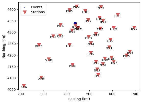
Let’s write out the 5 closest stations. The first four of those require special treatment:
# Distance from cluster centroid to stations
dists = utils.cartesian_distance(
    *evxyz.mean(axis=0), stxyz[:, 0], stxyz[:, 1], stxyz[:, 2]
)
idist = dists.argsort()

n = 5
print(f"The {n} closest stations are:")
for i in range(n):
    print(f"{stnames[idist[i]] :5s}: {dists[idist[i]]:.1f} km")
The 5 closest stations are:
EP10 : 14.3 km
EP08A: 26.4 km
EP08 : 27.2 km
EP09 : 35.8 km
EP07 : 59.6 km
We next define special data windows for the four closest stations. They are based on analyst experience on working with the data set at hand.
We then extract the waveform identifiers present in the phase dictionary. A waveform identifier refers to a combination of a station and a phase type and are characterized by a similar waveform.
# Special data windows
specialdw = {"EP10": 3.15, "EP08A": 6.25, "EP08": 6.25, "EP09": 6.5}

# Unique wave IDs in the phase dictionary
wvids = sorted(set(core.join_waveid(*core.split_phaseid(phid)[1:]) for phid in phd))
for wvid in wvids:

    # Station and phase
    sta, pha = core.split_waveid(wvid)

    # Initialize header
    hdr = core.Header()

    # Set station name and phase
    hdr["station"], hdr["phase"] = sta, pha

    # Apply special data window if needed
    if pha == "P" and sta in specialdw:
        hdr["data_window"] = specialdw[sta]
        hdr["phase_end"] = (specialdw[sta] - def_hdr["taper_length"] - 0.1) / 2
        hdr["highpass"] = 1  # Shorter time window requires higher highpass

    hdrf = core.file("waveform_header", sta, pha, directory="muji")
    hdr.to_file(hdrf, overwrite=True)

    print(f"Header for waveform {wvid} written to: {hdrf}   ", end="\r")
print("Done writing headers.                                           ")
INFO : Configuration written to: muji/data/BRC6_P-hdr.yaml
INFO : Configuration written to: muji/data/BRC6_S-hdr.yaml
INFO : Configuration written to: muji/data/CHE6_P-hdr.yaml
INFO : Configuration written to: muji/data/CHE6_S-hdr.yaml
INFO : Configuration written to: muji/data/EP01_P-hdr.yaml
INFO : Configuration written to: muji/data/EP01_S-hdr.yaml
INFO : Configuration written to: muji/data/EP02_P-hdr.yaml
INFO : Configuration written to: muji/data/EP02_S-hdr.yaml
INFO : Configuration written to: muji/data/EP03_P-hdr.yaml
INFO : Configuration written to: muji/data/EP03_S-hdr.yaml
INFO : Configuration written to: muji/data/EP04_P-hdr.yaml
INFO : Configuration written to: muji/data/EP04_S-hdr.yaml
INFO : Configuration written to: muji/data/EP05_P-hdr.yaml
INFO : Configuration written to: muji/data/EP05_S-hdr.yaml
INFO : Configuration written to: muji/data/EP06_P-hdr.yaml
Header for waveform BRC6_P written to: muji/data/BRC6_P-hdr.yaml
Header for waveform BRC6_S written to: muji/data/BRC6_S-hdr.yaml
Header for waveform CHE6_P written to: muji/data/CHE6_P-hdr.yaml
Header for waveform CHE6_S written to: muji/data/CHE6_S-hdr.yaml
Header for waveform EP01_P written to: muji/data/EP01_P-hdr.yaml
Header for waveform EP01_S written to: muji/data/EP01_S-hdr.yaml
Header for waveform EP02_P written to: muji/data/EP02_P-hdr.yaml
Header for waveform EP02_S written to: muji/data/EP02_S-hdr.yaml
Header for waveform EP03_P written to: muji/data/EP03_P-hdr.yaml
Header for waveform EP03_S written to: muji/data/EP03_S-hdr.yaml
Header for waveform EP04_P written to: muji/data/EP04_P-hdr.yaml
Header for waveform EP04_S written to: muji/data/EP04_S-hdr.yaml
Header for waveform EP05_P written to: muji/data/EP05_P-hdr.yaml
Header for waveform EP05_S written to: muji/data/EP05_S-hdr.yaml
Header for waveform EP06_P written to: muji/data/EP06_P-hdr.yaml
INFO : Configuration written to: muji/data/EP06_S-hdr.yaml
INFO : Configuration written to: muji/data/EP07_P-hdr.yaml
INFO : Configuration written to: muji/data/EP07_S-hdr.yaml
INFO : Configuration written to: muji/data/EP08A_P-hdr.yaml
INFO : Configuration written to: muji/data/EP08_P-hdr.yaml
INFO : Configuration written to: muji/data/EP08_S-hdr.yaml
INFO : Configuration written to: muji/data/EP09_P-hdr.yaml
INFO : Configuration written to: muji/data/EP09_S-hdr.yaml
INFO : Configuration written to: muji/data/EP10_P-hdr.yaml
INFO : Configuration written to: muji/data/EP10_S-hdr.yaml
INFO : Configuration written to: muji/data/EP11_P-hdr.yaml
INFO : Configuration written to: muji/data/EP11_S-hdr.yaml
INFO : Configuration written to: muji/data/EP12_P-hdr.yaml
INFO : Configuration written to: muji/data/EP13_P-hdr.yaml
INFO : Configuration written to: muji/data/EP13_S-hdr.yaml
INFO : Configuration written to: muji/data/EP14_P-hdr.yaml
INFO : Configuration written to: muji/data/EP14_S-hdr.yaml
INFO : Configuration written to: muji/data/EP15_P-hdr.yaml
INFO : Configuration written to: muji/data/EP15_S-hdr.yaml
INFO : Configuration written to: muji/data/EP16_P-hdr.yaml
INFO : Configuration written to: muji/data/EP16_S-hdr.yaml
INFO : Configuration written to: muji/data/EP17_P-hdr.yaml
INFO : Configuration written to: muji/data/EP18_P-hdr.yaml
INFO : Configuration written to: muji/data/EP18_S-hdr.yaml
INFO : Configuration written to: muji/data/EP19_P-hdr.yaml
INFO : Configuration written to: muji/data/EP19_S-hdr.yaml
INFO : Configuration written to: muji/data/EP20_P-hdr.yaml
INFO : Configuration written to: muji/data/EP21_P-hdr.yaml
INFO : Configuration written to: muji/data/EP21_S-hdr.yaml
INFO : Configuration written to: muji/data/EP22_P-hdr.yaml
INFO : Configuration written to: muji/data/EP22_S-hdr.yaml
INFO : Configuration written to: muji/data/EP23_P-hdr.yaml
INFO : Configuration written to: muji/data/EP24_P-hdr.yaml
INFO : Configuration written to: muji/data/EP24_S-hdr.yaml
INFO : Configuration written to: muji/data/EP25_P-hdr.yaml
INFO : Configuration written to: muji/data/EP25_S-hdr.yaml
INFO : Configuration written to: muji/data/EP27_P-hdr.yaml
INFO : Configuration written to: muji/data/EP28_P-hdr.yaml
INFO : Configuration written to: muji/data/EP29_P-hdr.yaml
INFO : Configuration written to: muji/data/EP30_P-hdr.yaml
INFO : Configuration written to: muji/data/ICE6_P-hdr.yaml
INFO : Configuration written to: muji/data/ICE6_S-hdr.yaml
INFO : Configuration written to: muji/data/ISH6_P-hdr.yaml
INFO : Configuration written to: muji/data/LAN6_P-hdr.yaml
INFO : Configuration written to: muji/data/LAN6_S-hdr.yaml
INFO : Configuration written to: muji/data/P116_P-hdr.yaml
INFO : Configuration written to: muji/data/P116_S-hdr.yaml
INFO : Configuration written to: muji/data/P146_P-hdr.yaml
INFO : Configuration written to: muji/data/P146_S-hdr.yaml
INFO : Configuration written to: muji/data/P236_P-hdr.yaml
INFO : Configuration written to: muji/data/P236_S-hdr.yaml
INFO : Configuration written to: muji/data/SUM6_P-hdr.yaml
INFO : Configuration written to: muji/data/SUM6_S-hdr.yaml
Header for waveform EP06_S written to: muji/data/EP06_S-hdr.yaml
Header for waveform EP07_P written to: muji/data/EP07_P-hdr.yaml
Header for waveform EP07_S written to: muji/data/EP07_S-hdr.yaml
Header for waveform EP08A_P written to: muji/data/EP08A_P-hdr.yaml
Header for waveform EP08_P written to: muji/data/EP08_P-hdr.yaml
Header for waveform EP08_S written to: muji/data/EP08_S-hdr.yaml
Header for waveform EP09_P written to: muji/data/EP09_P-hdr.yaml
Header for waveform EP09_S written to: muji/data/EP09_S-hdr.yaml
Header for waveform EP10_P written to: muji/data/EP10_P-hdr.yaml
Header for waveform EP10_S written to: muji/data/EP10_S-hdr.yaml
Header for waveform EP11_P written to: muji/data/EP11_P-hdr.yaml
Header for waveform EP11_S written to: muji/data/EP11_S-hdr.yaml
Header for waveform EP12_P written to: muji/data/EP12_P-hdr.yaml
Header for waveform EP13_P written to: muji/data/EP13_P-hdr.yaml
Header for waveform EP13_S written to: muji/data/EP13_S-hdr.yaml
Header for waveform EP14_P written to: muji/data/EP14_P-hdr.yaml
Header for waveform EP14_S written to: muji/data/EP14_S-hdr.yaml
Header for waveform EP15_P written to: muji/data/EP15_P-hdr.yaml
Header for waveform EP15_S written to: muji/data/EP15_S-hdr.yaml
Header for waveform EP16_P written to: muji/data/EP16_P-hdr.yaml
Header for waveform EP16_S written to: muji/data/EP16_S-hdr.yaml
Header for waveform EP17_P written to: muji/data/EP17_P-hdr.yaml
Header for waveform EP18_P written to: muji/data/EP18_P-hdr.yaml
Header for waveform EP18_S written to: muji/data/EP18_S-hdr.yaml
Header for waveform EP19_P written to: muji/data/EP19_P-hdr.yaml
Header for waveform EP19_S written to: muji/data/EP19_S-hdr.yaml
Header for waveform EP20_P written to: muji/data/EP20_P-hdr.yaml
Header for waveform EP21_P written to: muji/data/EP21_P-hdr.yaml
Header for waveform EP21_S written to: muji/data/EP21_S-hdr.yaml
Header for waveform EP22_P written to: muji/data/EP22_P-hdr.yaml
Header for waveform EP22_S written to: muji/data/EP22_S-hdr.yaml
Header for waveform EP23_P written to: muji/data/EP23_P-hdr.yaml
Header for waveform EP24_P written to: muji/data/EP24_P-hdr.yaml
Header for waveform EP24_S written to: muji/data/EP24_S-hdr.yaml
Header for waveform EP25_P written to: muji/data/EP25_P-hdr.yaml
Header for waveform EP25_S written to: muji/data/EP25_S-hdr.yaml
Header for waveform EP27_P written to: muji/data/EP27_P-hdr.yaml
Header for waveform EP28_P written to: muji/data/EP28_P-hdr.yaml
Header for waveform EP29_P written to: muji/data/EP29_P-hdr.yaml
Header for waveform EP30_P written to: muji/data/EP30_P-hdr.yaml
Header for waveform ICE6_P written to: muji/data/ICE6_P-hdr.yaml
Header for waveform ICE6_S written to: muji/data/ICE6_S-hdr.yaml
Header for waveform ISH6_P written to: muji/data/ISH6_P-hdr.yaml
Header for waveform LAN6_P written to: muji/data/LAN6_P-hdr.yaml
Header for waveform LAN6_S written to: muji/data/LAN6_S-hdr.yaml
Header for waveform P116_P written to: muji/data/P116_P-hdr.yaml
Header for waveform P116_S written to: muji/data/P116_S-hdr.yaml
Header for waveform P146_P written to: muji/data/P146_P-hdr.yaml
Header for waveform P146_S written to: muji/data/P146_S-hdr.yaml
Header for waveform P236_P written to: muji/data/P236_P-hdr.yaml
Header for waveform P236_S written to: muji/data/P236_S-hdr.yaml
Header for waveform SUM6_P written to: muji/data/SUM6_P-hdr.yaml
Header for waveform SUM6_S written to: muji/data/SUM6_S-hdr.yaml
Done writing headers.
Construct the waveform arrays#
The waveform arrays hold the waveform data and are central to relMT. They are of shape (events, channels, samples). The dimensions must be in agreement with the values of the header values "events_", "channels", "data_window" and "sampling_rate".
We now set up the waveform array for each seismic station and phase in the data set. We loop through the header files we just created. The "events_" keyword needs special attention because each seismic station in general recorded a different set of events.
from numpy import save
from obspy import read
from pathlib import Path

# Project directory
projdir = "muji"

# Waveform directory
wvdir = Path("ext")

# Load MiniSEED wavforms into ObsPy Stream
stream = read(wvdir / "*.mseed")

# Unique wave IDs in the phase dictionary
wvids = sorted(set(core.join_waveid(*core.split_phaseid(phid)[1:]) for phid in phd))

# Default values are read from the default header file
default_hdrf = core.file("waveform_header", directory=projdir)

for wvid in wvids:
    print(f"Processing waveform {wvid}...", end="\r")

    # Station and phase
    sta, pha = core.split_waveid(wvid)

    # core.file implements the naming convention for relMT files
    hdrf = core.file("waveform_header", sta, pha, directory=projdir)
    arrf = core.file("waveform_array", sta, pha, directory=projdir)

    # Read the header, filling in defaults where necessary
    hdr = io.read_header(hdrf, default_hdrf)

    wvarr, hdr = extra.make_waveform_array(hdr, phd, stream)

    # Waveform arrays are conventional .npy files
    save(arrf, wvarr)

    # We write the specific waveform header
    hdr.to_file(hdrf, overwrite=True)

# List the created waveform array files
! ls muji/data/*-wvarr.npy
Processing waveform BRC6_P...
INFO : Configuration written to: muji/data/BRC6_P-hdr.yaml
Processing waveform BRC6_S...
INFO : Configuration written to: muji/data/BRC6_S-hdr.yaml
Processing waveform CHE6_P...
INFO : Configuration written to: muji/data/CHE6_P-hdr.yaml
Processing waveform CHE6_S...
INFO : Configuration written to: muji/data/CHE6_S-hdr.yaml
Processing waveform EP01_P...
INFO : Configuration written to: muji/data/EP01_P-hdr.yaml
Processing waveform EP01_S...
INFO : Configuration written to: muji/data/EP01_S-hdr.yaml
Processing waveform EP02_P...
INFO : Configuration written to: muji/data/EP02_P-hdr.yaml
Processing waveform EP02_S...
INFO : Configuration written to: muji/data/EP02_S-hdr.yaml
Processing waveform EP03_P...
INFO : Configuration written to: muji/data/EP03_P-hdr.yaml
Processing waveform EP03_S...
INFO : Configuration written to: muji/data/EP03_S-hdr.yaml
Processing waveform EP04_P...
INFO : Configuration written to: muji/data/EP04_P-hdr.yaml
Processing waveform EP04_S...
INFO : Configuration written to: muji/data/EP04_S-hdr.yaml
Processing waveform EP05_P...
INFO : Configuration written to: muji/data/EP05_P-hdr.yaml
Processing waveform EP05_S...
INFO : Configuration written to: muji/data/EP05_S-hdr.yaml
Processing waveform EP06_P...
INFO : Configuration written to: muji/data/EP06_P-hdr.yaml
Processing waveform EP06_S...
INFO : Configuration written to: muji/data/EP06_S-hdr.yaml
Processing waveform EP07_P...
INFO : Configuration written to: muji/data/EP07_P-hdr.yaml
Processing waveform EP07_S...
INFO : Configuration written to: muji/data/EP07_S-hdr.yaml
Processing waveform EP08A_P...
INFO : Configuration written to: muji/data/EP08A_P-hdr.yaml
INFO : Configuration written to: muji/data/EP08_P-hdr.yaml
INFO : Configuration written to: muji/data/EP08_S-hdr.yaml
Processing waveform EP08_P...
Processing waveform EP08_S...
Processing waveform EP09_P...
INFO : Configuration written to: muji/data/EP09_P-hdr.yaml
Processing waveform EP09_S...
INFO : Configuration written to: muji/data/EP09_S-hdr.yaml
Processing waveform EP10_P...
INFO : Configuration written to: muji/data/EP10_P-hdr.yaml
Processing waveform EP10_S...
INFO : Configuration written to: muji/data/EP10_S-hdr.yaml
Processing waveform EP11_P...
INFO : Configuration written to: muji/data/EP11_P-hdr.yaml
Processing waveform EP11_S...
INFO : Configuration written to: muji/data/EP11_S-hdr.yaml
INFO : Configuration written to: muji/data/EP12_P-hdr.yaml
Processing waveform EP12_P...
Processing waveform EP13_P...
INFO : Configuration written to: muji/data/EP13_P-hdr.yaml
Processing waveform EP13_S...
INFO : Configuration written to: muji/data/EP13_S-hdr.yaml
Processing waveform EP14_P...
INFO : Configuration written to: muji/data/EP14_P-hdr.yaml
Processing waveform EP14_S...
INFO : Configuration written to: muji/data/EP14_S-hdr.yaml
Processing waveform EP15_P...
INFO : Configuration written to: muji/data/EP15_P-hdr.yaml
Processing waveform EP15_S...
INFO : Configuration written to: muji/data/EP15_S-hdr.yaml
Processing waveform EP16_P...
INFO : Configuration written to: muji/data/EP16_P-hdr.yaml
Processing waveform EP16_S...
INFO : Configuration written to: muji/data/EP16_S-hdr.yaml
INFO : Configuration written to: muji/data/EP17_P-hdr.yaml
Processing waveform EP17_P...
Processing waveform EP18_P...
INFO : Configuration written to: muji/data/EP18_P-hdr.yaml
Processing waveform EP18_S...
INFO : Configuration written to: muji/data/EP18_S-hdr.yaml
Processing waveform EP19_P...
INFO : Configuration written to: muji/data/EP19_P-hdr.yaml
Processing waveform EP19_S...
INFO : Configuration written to: muji/data/EP19_S-hdr.yaml
INFO : Configuration written to: muji/data/EP20_P-hdr.yaml
Processing waveform EP20_P...
Processing waveform EP21_P...
INFO : Configuration written to: muji/data/EP21_P-hdr.yaml
Processing waveform EP21_S...
INFO : Configuration written to: muji/data/EP21_S-hdr.yaml
Processing waveform EP22_P...
INFO : Configuration written to: muji/data/EP22_P-hdr.yaml
Processing waveform EP22_S...
INFO : Configuration written to: muji/data/EP22_S-hdr.yaml
INFO : Configuration written to: muji/data/EP23_P-hdr.yaml
Processing waveform EP23_P...
Processing waveform EP24_P...
INFO : Configuration written to: muji/data/EP24_P-hdr.yaml
Processing waveform EP24_S...
INFO : Configuration written to: muji/data/EP24_S-hdr.yaml
Processing waveform EP25_P...
INFO : Configuration written to: muji/data/EP25_P-hdr.yaml
Processing waveform EP25_S...
INFO : Configuration written to: muji/data/EP25_S-hdr.yaml
INFO : Configuration written to: muji/data/EP27_P-hdr.yaml
Processing waveform EP27_P...
Processing waveform EP28_P...
INFO : Configuration written to: muji/data/EP28_P-hdr.yaml
Processing waveform EP29_P...
INFO : Configuration written to: muji/data/EP29_P-hdr.yaml
Processing waveform EP30_P...
INFO : Configuration written to: muji/data/EP30_P-hdr.yaml
INFO : Configuration written to: muji/data/ICE6_P-hdr.yaml
INFO : Configuration written to: muji/data/ICE6_S-hdr.yaml
Processing waveform ICE6_P...
Processing waveform ICE6_S...
Processing waveform ISH6_P...
INFO : Configuration written to: muji/data/ISH6_P-hdr.yaml
Processing waveform LAN6_P...
INFO : Configuration written to: muji/data/LAN6_P-hdr.yaml
Processing waveform LAN6_S...
INFO : Configuration written to: muji/data/LAN6_S-hdr.yaml
Processing waveform P116_P...
INFO : Configuration written to: muji/data/P116_P-hdr.yaml
Processing waveform P116_S...
INFO : Configuration written to: muji/data/P116_S-hdr.yaml
INFO : Configuration written to: muji/data/P146_P-hdr.yaml
INFO : Configuration written to: muji/data/P146_S-hdr.yaml
Processing waveform P146_P...
Processing waveform P146_S...
Processing waveform P236_P...
INFO : Configuration written to: muji/data/P236_P-hdr.yaml
Processing waveform P236_S...
INFO : Configuration written to: muji/data/P236_S-hdr.yaml
Processing waveform SUM6_P...
INFO : Configuration written to: muji/data/SUM6_P-hdr.yaml
Processing waveform SUM6_S...
INFO : Configuration written to: muji/data/SUM6_S-hdr.yaml
muji/data/BRC6_P-wvarr.npy   muji/data/EP16_P-wvarr.npy
muji/data/BRC6_S-wvarr.npy   muji/data/EP16_S-wvarr.npy
muji/data/CHE6_P-wvarr.npy   muji/data/EP17_P-wvarr.npy
muji/data/CHE6_S-wvarr.npy   muji/data/EP18_P-wvarr.npy
muji/data/EP01_P-wvarr.npy   muji/data/EP18_S-wvarr.npy
muji/data/EP01_S-wvarr.npy   muji/data/EP19_P-wvarr.npy
muji/data/EP02_P-wvarr.npy   muji/data/EP19_S-wvarr.npy
muji/data/EP02_S-wvarr.npy   muji/data/EP20_P-wvarr.npy
muji/data/EP03_P-wvarr.npy   muji/data/EP21_P-wvarr.npy
muji/data/EP03_S-wvarr.npy   muji/data/EP21_S-wvarr.npy
muji/data/EP04_P-wvarr.npy   muji/data/EP22_P-wvarr.npy
muji/data/EP04_S-wvarr.npy   muji/data/EP22_S-wvarr.npy
muji/data/EP05_P-wvarr.npy   muji/data/EP23_P-wvarr.npy
muji/data/EP05_S-wvarr.npy   muji/data/EP24_P-wvarr.npy
muji/data/EP06_P-wvarr.npy   muji/data/EP24_S-wvarr.npy
muji/data/EP06_S-wvarr.npy   muji/data/EP25_P-wvarr.npy
muji/data/EP07_P-wvarr.npy   muji/data/EP25_S-wvarr.npy
muji/data/EP07_S-wvarr.npy   muji/data/EP27_P-wvarr.npy
muji/data/EP08A_P-wvarr.npy  muji/data/EP28_P-wvarr.npy
muji/data/EP08_P-wvarr.npy   muji/data/EP29_P-wvarr.npy
muji/data/EP08_S-wvarr.npy   muji/data/EP30_P-wvarr.npy
muji/data/EP09_P-wvarr.npy   muji/data/ICE6_P-wvarr.npy
muji/data/EP09_S-wvarr.npy   muji/data/ICE6_S-wvarr.npy
muji/data/EP10_P-wvarr.npy   muji/data/ISH6_P-wvarr.npy
muji/data/EP10_S-wvarr.npy   muji/data/LAN6_P-wvarr.npy
muji/data/EP11_P-wvarr.npy   muji/data/LAN6_S-wvarr.npy
muji/data/EP11_S-wvarr.npy   muji/data/P116_P-wvarr.npy
muji/data/EP12_P-wvarr.npy   muji/data/P116_S-wvarr.npy
muji/data/EP13_P-wvarr.npy   muji/data/P146_P-wvarr.npy
muji/data/EP13_S-wvarr.npy   muji/data/P146_S-wvarr.npy
muji/data/EP14_P-wvarr.npy   muji/data/P236_P-wvarr.npy
muji/data/EP14_S-wvarr.npy   muji/data/P236_S-wvarr.npy
muji/data/EP15_P-wvarr.npy   muji/data/SUM6_P-wvarr.npy
muji/data/EP15_S-wvarr.npy   muji/data/SUM6_S-wvarr.npy
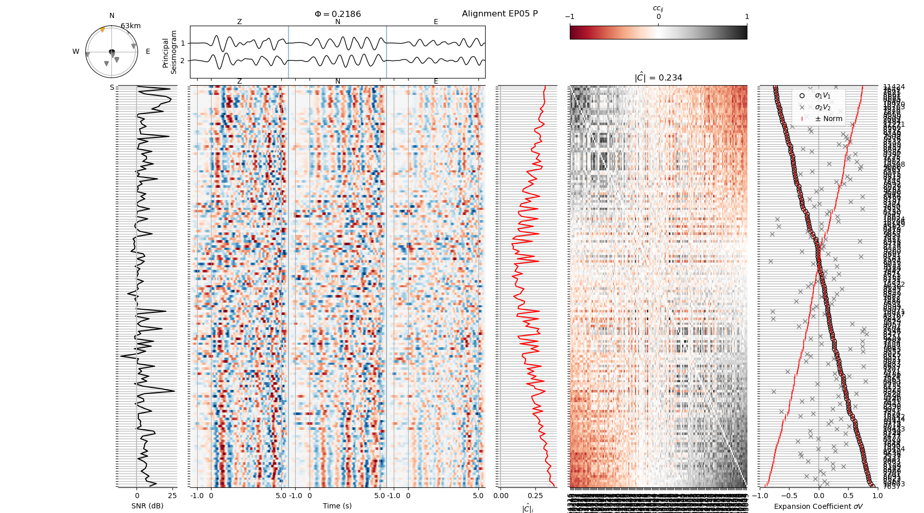
Conclusion#
In this example we extracted an event subset from a large earthquake catalog and downloaded station and waveform data from publicly accessible repository. Let’s have a look at the P waveform recorded on station EP05:
# Plot an example waveform alignment
# On the command line, one can omit the --saveas option to show an interactive plot
! relmt plot-alignment muji/data/EP05_P-wvarr.npy -c muji/config.yaml --saveas tmp.png

# Show and clean up in the notebook
display(Image("tmp.png"))
! rm tmp.png
INFO : Computing correlation coefficients of all event combinations. This may take a while...